Lesson 39: TEE Review

Canvas Turn-In – Due Today

Submit both of the following on Canvas as two separate submissions:

Project Presentation – upload to the Project Presentation submission slot
Technical Report – upload to the Tech Report submission slot

TEE Logistics

TEE Schedule

Section	12 May 0730–1100	13 May 0730–1100	15 May 1300–1630
A2	2	0	15
B2	1	0	17
C2	3	1	12

Full Section Roster by Date

12 May, 0730–1100

EDDY, ELLIOT G
HARDER, ETHAN W
JENKINS, KEIRA M
KALIDINDI, HEERA S
NEWTON, SEAN J

13 May, 0730–1100

PHELPS, JOHN M

15 May, 1300–1630

AIRD, ZANDER A
ASHLEY, CAIDEN E
BOOZER, CURTIS M
CARTER, ISAAC M
DWYER, LUKE P
GARMON, MICHAEL H
HOLTMAN, ETHAN M
KELLY, BRENDAN R
MCFARREN, SYDNEY L
MCGREGOR, AUSTYN J
MERIDETH, JUDSON W
O’CONNOR, OWEN W

12 May, 0730–1100

FEDALIZO, BALTAZAR C

13 May, 0730–1100

WEGNER, DYLAN D

15 May, 1300–1630

BARTOSH, BRIGHAM A
CHEN, JUSTIN R
CUETO, NICHOLAS C
DIOP, KHADIJA
GRIFFIN, CAMERON J
HEKIMIAN, MARY RAY M
ISONIEMI, JONATHAN A
JEFFREY, ALEXANDER M
KIM, DOYEE
LEDFORD, PEYTON R
LEE, CALEB S
MAESTAS, NATHAN J
MULHOLLAND, THOMAS P
NEWMAN, NICHOLAS P
RIBAS, HELEN A
ROSS, JAMES C

12 May, 0730–1100

CALABRESE, BENJAMIN C
HONG, RAYMOND
KWAK, TREVOR J

13 May, 0730–1100

GRAY, WILLIAM C

15 May, 1300–1630

BANZUELA, JOSHUA M
BRADLEY, GAVIN M
BRAEGER, SYDNEY M
CASTINO, RYLEN J
CATALDO, JUSTIN J
DIAL, NADIA J
HARTLEY, JETT M
LINEBERGER, JAYDEN D
PAYNE, BRENNA N
POULTER, ZANE C
PRATT, NATHAN C
PROKOP, ANYA A

What you can bring

Reference card (the SRC – linked below). Print it; bring it to the test.
Calculator.
R-lite for distribution functions (pnorm/qnorm, pt/qt, pbinom, ppois, pexp, pf/qf).

TEE Review Materials

Download these now

TEE materials

TEE Review (Practice Problems) – comprehensive review covering everything on the TEE
TEE Review – Solutions – worked solutions to every problem in the review
Student Reference Card (SRC) – the formula sheet you may bring into the TEE
R-Lite (updated) – the standalone R distribution-function tool you may use on the TEE

WPR I materials (Lessons 1–14: data, probability, random variables, distributions)

WPR II materials (Lessons 17–25: CLT, CIs, hypothesis tests, two-sample inference)

You need this updated version of R-Lite

The R-Lite executable linked above has been updated – earlier copies you downloaded during the semester are out of date. Download this version and use it for the TEE. It’s the only R-Lite that will be permitted in the testing room.

How to use these materials. Work the Review closed-book with only the SRC, your calculator, and R-lite. After you finish a section, check your work against the Solutions. If you missed something, go back to the lesson(s) for that topic in the outline below.

Course Outline – Everything We Did

The course was organized into three blocks. Every topic listed here is fair game on the TEE; the TEE Review covers them all.

Block I: Data and Randomness (Lessons 1–16)

L1–5: Types of Data, Sampling, Study Design (Devore 1.1–1.4, 2.1–2.2)
- Populations vs. samples vs. processes; parameters vs. statistics
- Categorical vs. quantitative variables
- Observational studies vs. designed experiments
- Common sampling methods and biases; randomization and control
L6–8: Measures of Location and Variability (Devore 2.3–2.5, 3.1–3.6)
- Mean, median, mode; percentiles and quartiles
- Range, IQR, variance, standard deviation
L9: Exploratory Data Analysis (Devore 4.1–4.3)
- Choosing displays for variable types; communicating findings
L10–11: Probability Basics
- Kolmogorov axioms
- Inclusion–Exclusion: $P(A \cup B) = P(A) + P(B) - P(A \cap B)$
- Complement, mutually exclusive vs. independent
L12: Conditional Probability and Independence
- $P(A \mid B) = \dfrac{P(A \cap B)}{P(B)}$
- Multiplication rule; Bayes’ Rule and the Law of Total Probability
- Counting: ordered/unordered, with/without replacement
L13: Discrete Random Variables (Devore 4.4)
- PMFs, CDFs; $E[X]$, $V[X]$
L14: Binomial and Poisson
- Binomial: counts of successes in $n$ Bernoulli trials. $E[X] = np$, $V[X] = np(1-p)$
- Poisson: counts of rare events at rate $\lambda$. $E[X] = V[X] = \lambda$
- Poisson approximation to binomial when $n$ large, $p$ small
L15: Continuous Random Variables (Normal, Exponential) (Devore 5.3–5.4)
- pdfs and cdfs; $P(X = c) = 0$ for continuous $X$
- Normal: standardize with $Z = (X - \mu)/\sigma$
- Exponential: rate $\lambda$, mean $1/\lambda$, memoryless property
L16: WPR I – covered Lessons 1–14

Block II: Inference (Lessons 17–27)

L17: Central Limit Theorem (Devore 7.1–7.3)
- Sampling distribution of $\bar{X}$ is approximately $N\!\left(\mu,\,\sigma^2/n\right)$ for large $n$
- Same for $\hat{p}$ when $np \ge 10$ and $n(1-p) \ge 10$
L18–19: Confidence Intervals
- One-sample CI for $\mu$: $\bar{x} \pm t_{\alpha/2,\,n-1}\,s/\sqrt{n}$
- One-sample CI for $p$: $\hat{p} \pm z_{\alpha/2}\sqrt{\hat{p}(1-\hat{p})/n}$
- Margin of error, sample-size determination
- Correct interpretation: “If we repeated the procedure many times, $(1-\alpha)$ of the resulting intervals would contain the true parameter.”
L20–21: Hypothesis Testing and One-Sample t-Test
- $H_0$ vs. $H_a$; test statistic; p-value
- Type I ($\alpha$) and Type II ($\beta$) error; power $= 1 - \beta$
- One-sample t: $t = \dfrac{\bar{x} - \mu_0}{s/\sqrt{n}}$ on $n-1$ df
L22: One-Proportion z-Test
- $z = \dfrac{\hat{p} - p_0}{\sqrt{p_0(1-p_0)/n}}$
- Practical vs. statistical significance
L23: Two-Sample t-Test (Independent)
- Welch’s t (default); pooled when variances are equal
- $t = \dfrac{\bar{x}_1 - \bar{x}_2}{\sqrt{s_1^2/n_1 + s_2^2/n_2}}$
- Conservative df: $\min(n_1 - 1,\, n_2 - 1)$
L24: Paired t-Test
- Compute differences $d_i = x_{1i} - x_{2i}$, then run a one-sample t on the differences
- Choose paired vs. independent based on study design
L25: Two-Proportion z-Test
- Pooled SE for the test, unpooled SE for the CI
- $z = \dfrac{\hat{p}_1 - \hat{p}_2}{\sqrt{\hat{p}(1-\hat{p})(1/n_1 + 1/n_2)}}$ where $\hat{p}$ is the pooled proportion
L26–27: Review and WPR II – covered Lessons 17–25

Block III: Regression and ANOVA (Lessons 28–38)

L28, L30: Simple Linear Regression (Devore 12.1–12.5)
- Least-squares line: $\hat{y} = b_0 + b_1 x$
- $R^2$ = proportion of variability in $y$ explained by the model
- $t$-test for slope; CIs for $\beta_1$
- Mean-response CI vs. prediction interval
- Don’t extrapolate beyond the range of $x$
L31–33: Multiple Linear Regression
- Coefficient interpretation: change in $y$ per one-unit increase in $x_j$, holding all other predictors constant
- Adjusted $R^2$ for model selection
- Indicator (dummy) variables for categorical predictors
- Interaction terms; main effects vs. interaction effects
- Confounding and threats to causal inference
L34–35: Project Peer Review and Lecture Drop – Tech Report due Lesson 36
L36–37: ANOVA (Devore 10.1–10.2)
- One-way ANOVA hypotheses: $H_0: \mu_1 = \cdots = \mu_k$
- $F = MSTr / MSE$ on $(k-1,\,N-k)$ df
- Tukey’s HSD for which pairs differ; family-wise error rate
L38: Project Presentations

Reference Tables

Printable PDF

The wide tables below are easier to read on paper. Download:

Inference Summary (PDF, landscape) – hypothesis tests + CIs in one place.

Named Distributions

Distribution	Type	Notation	Mean	Variance
Binomial	Discrete	$X \sim \text{Bin}(n, p)$	$np$	$np(1-p)$
Poisson	Discrete	$X \sim \text{Pois}(\lambda)$	$\lambda$	$\lambda$
Normal	Continuous	$X \sim N(\mu, \sigma^2)$	$\mu$	$\sigma^2$
Exponential	Continuous	$X \sim \text{Exp}(\lambda)$	$1/\lambda$	$1/\lambda^2$

Summary of Hypothesis Tests

	One-Sample Mean (Large)	One-Sample Mean (Small)	One Proportion	Two-Sample Mean (Large)	Two-Sample Mean (Small)	Paired Mean	Two Proportions	One-Way ANOVA
Parameter	$\mu$	$\mu$	$p$	$\mu_1 - \mu_2$	$\mu_1 - \mu_2$	$\mu_d$	$p_1 - p_2$	$\mu_1, \dots, \mu_k$
$H_0$	$\mu = \mu_0$	$\mu = \mu_0$	$p = p_0$	$\mu_1 - \mu_2 = \Delta_0$	$\mu_1 - \mu_2 = \Delta_0$	$\mu_d = \Delta_0$	$p_1 - p_2 = 0$	$\mu_1 = \cdots = \mu_k$
$H_a$	$\mu \neq, <, > \mu_0$	$\mu \neq, <, > \mu_0$	$p \neq, <, > p_0$	$\mu_1 - \mu_2 \neq, <, > 0$	$\mu_1 - \mu_2 \neq, <, > 0$	$\mu_d \neq, <, > 0$	$p_1 - p_2 \neq, <, > 0$	at least one $\mu_i$ differs
Test Statistic	$z = \dfrac{\bar{x} - \mu_0}{\sigma / \sqrt{n}}$	$t = \dfrac{\bar{x} - \mu_0}{s / \sqrt{n}}$	$z = \dfrac{\hat{p} - p_0}{\sqrt{p_0(1-p_0)/n}}$	$z = \dfrac{\bar{x}_1 - \bar{x}_2}{\sqrt{s_1^2/n_1 + s_2^2/n_2}}$	$t = \dfrac{\bar{x}_1 - \bar{x}_2}{\sqrt{s_1^2/n_1 + s_2^2/n_2}}$	$t = \dfrac{\bar{d} - \Delta_0}{s_d / \sqrt{n}}$	$z = \dfrac{\hat{p}_1 - \hat{p}_2}{\sqrt{\hat{p}(1-\hat{p})(1/n_1 + 1/n_2)}}$	$F = \dfrac{MSTr}{MSE}$
Distribution	$N(0,1)$	$t_{n-1}$	$N(0,1)$	$N(0,1)$	$t_{\min(n_1-1, n_2-1)}$	$t_{n-1}$	$N(0,1)$	$F_{k-1,\,N-k}$
Left-tailed $p$	`pnorm(z)`	`pt(t, df)`	`pnorm(z)`	`pnorm(z)`	`pt(t, df)`	`pt(t, df)`	`pnorm(z)`	–
Right-tailed $p$	`1 - pnorm(z)`	`1 - pt(t, df)`	`1 - pnorm(z)`	`1 - pnorm(z)`	`1 - pt(t, df)`	`1 - pt(t, df)`	`1 - pnorm(z)`	`1 - pf(F, df1, df2)`
Two-tailed $p$	`2*(1 - pnorm(abs(z)))`	`2*(1 - pt(abs(t), df))`	`2*(1 - pnorm(abs(z)))`	`2*(1 - pnorm(abs(z)))`	`2*(1 - pt(abs(t), df))`	`2*(1 - pt(abs(t), df))`	`2*(1 - pnorm(abs(z)))`	–
Conditions	$n \geq 30$	Normal pop or $n \geq 30$	$np_0 \geq 10$ & $n(1-p_0) \geq 10$	$n_1, n_2 \geq 30$	Both pops $\sim$ Normal	Diffs $\sim$ Normal or $n \geq 30$	$n_i\hat{p}_i \geq 10$ & $n_i(1-\hat{p}_i) \geq 10$	Indep. samples; equal-variance, approx. normal within groups

Decision rule is always the same: $p \leq \alpha$ → Reject $H_0$. $p > \alpha$ → Fail to reject $H_0$.

Summary of Confidence Intervals

	One-Sample Mean (Large)	One-Sample Mean (Small)	One Proportion	Two-Sample Mean	Paired Mean	Two Proportions
Parameter	$\mu$	$\mu$	$p$	$\mu_1 - \mu_2$	$\mu_d$	$p_1 - p_2$
Formula	$\bar{x} \pm z_{\alpha/2} \cdot \dfrac{\sigma}{\sqrt{n}}$	$\bar{x} \pm t_{\alpha/2,\, n-1} \cdot \dfrac{s}{\sqrt{n}}$	$\hat{p} \pm z_{\alpha/2} \cdot \sqrt{\dfrac{\hat{p}(1-\hat{p})}{n}}$	$(\bar{x}_1 - \bar{x}_2) \pm t_{\alpha/2} \cdot \sqrt{\dfrac{s_1^2}{n_1} + \dfrac{s_2^2}{n_2}}$	$\bar{d} \pm t_{\alpha/2,\, n-1} \cdot \dfrac{s_d}{\sqrt{n}}$	$(\hat{p}_1 - \hat{p}_2) \pm z_{\alpha/2} \cdot \sqrt{\dfrac{\hat{p}_1(1-\hat{p}_1)}{n_1} + \dfrac{\hat{p}_2(1-\hat{p}_2)}{n_2}}$
Conditions	$n \geq 30$	Normal pop or $n \geq 30$	$n\hat{p} \geq 10$ & $n(1-\hat{p}) \geq 10$	$n_1, n_2 \geq 30$ (or Normal pops)	Diffs $\sim$ Normal or $n \geq 30$	$n_i\hat{p}_i \geq 10$ & $n_i(1-\hat{p}_i) \geq 10$

Possible Pitfalls

The traps that catch the most points

CI interpretation: “95% of the resulting intervals would contain the true parameter.” Not “95% probability the parameter is in this interval,” and not “95% of the population falls in this interval.”
p-value: probability of data at least as extreme as observed, assuming $H_0$ is true – not the probability $H_0$ is true.
Failing to reject $\ne$ accepting: “insufficient evidence to reject $H_0$” is the right phrasing.
MLR coefficients: always include “holding the other predictors constant.”
Don’t extrapolate a regression beyond the range of the observed predictors.
Continuous RVs: $P(X = c) = 0$ exactly, not “approximately.”
Mutually exclusive $\ne$ independent. Mutually exclusive events with positive probability are dependent.
Paired vs. independent: if subjects/units are matched (before/after, twins, same plot), it’s paired. Otherwise it’s independent.
Pooled vs. unpooled SE for two proportions: pool for the test, don’t pool for the CI.
ANOVA degrees of freedom: $F$ on $(k-1,\,N-k)$.

Break!

Reese

Cal

Worked Examples

Bayes’ Theorem – The Eyewitness Cab Problem

A taxicab is involved in a hit-and-run accident at night. Two cab companies serve the city:

Green Cab Co. operates 85% of the cabs.
Blue Cab Co. operates the remaining 15%.

A witness identifies the cab as Blue. The court tests the witness’s reliability under the same nighttime conditions and finds the witness correctly identifies a cab’s color 80% of the time and is wrong 20% of the time (regardless of whether the cab is actually Green or Blue).

Setup.

$B$ = cab is actually Blue
$G$ = cab is actually Green
$\hat{B}$ = witness identifies cab as Blue
$P(B) = 0.15$, $P(G) = 0.85$
$P(\hat{B} \mid B) = 0.80$
$P(\hat{B} \mid G) = 0.20$

(a) What is the probability that the witness identifies a randomly selected cab as Blue?

Solution (a). By the Law of Total Probability:

\[P(\hat{B}) = P(\hat{B} \mid B)P(B) + P(\hat{B} \mid G)P(G) = (0.80)(0.15) + (0.20)(0.85) = 0.12 + 0.17 = 0.29\]

(b) Given the witness identified the cab as Blue, what is the probability the cab actually was Blue?

Solution (b). By Bayes’ Theorem:

\[P(B \mid \hat{B}) = \frac{P(\hat{B} \mid B) P(B)}{P(\hat{B})} = \frac{(0.80)(0.15)}{0.29} = \frac{0.12}{0.29} \approx 0.414\]

Even with an 80%-reliable witness who says the cab was Blue, there is only about a 41% chance the cab really was Blue. Walk through 100 cabs:

15 are Blue → witness correctly flags 12 as “Blue”
85 are Green → witness mistakenly flags 17 as “Blue”
Of 29 total “Blue” calls, only $12/29 \approx 41\%$ are actually Blue

(This is the classic Tversky–Kahneman taxicab problem – a famous demonstration of base-rate neglect.)

Exponential and Poisson – Tactical Radio Net

Messages on a tactical radio net arrive randomly and independently at an average rate of 3 messages per 10 minutes. Two natural ways to model this same process:

The time between consecutive messages follows an exponential distribution.
The number of messages in a fixed window follows a Poisson distribution.

Setup. Let $T$ = time (in minutes) until the next message and $X$ = number of messages in a 10-minute window. The rate is 3 messages per 10 minutes, i.e., $\lambda = 0.3$ messages/minute.

(a) Identify the distribution of $T$ and state its rate parameter $\lambda$. Give $E[T]$ and $V[T]$.

Solution (a).

$T \sim \text{Exp}(\lambda = 0.3)$ per minute
$E[T] = 1/\lambda = 1/0.3 \approx 3.33$ min
$V[T] = 1/\lambda^2 = 1/0.09 \approx 11.11$ min$^2$

(b) Compute $P(T \le 4)$ – the probability the next message arrives within 4 minutes.

Solution (b). $P(T \le 4) = 1 - e^{-\lambda \cdot 4} = 1 - e^{-1.2} \approx 1 - 0.3012 = 0.6988$. R-lite: pexp(4, rate = 0.3) $\approx 0.6988$.

(c) Compute $P(T > 8)$ – the probability more than 8 minutes pass with no messages.

Solution (c). $P(T > 8) = e^{-0.3 \cdot 8} = e^{-2.4} \approx 0.0907$. R-lite: 1 - pexp(8, rate = 0.3) $\approx 0.0907$.

(d) Now flip to the count perspective. Identify the distribution of $X$ (messages in 10 minutes) and state its parameter. Give $E[X]$ and $V[X]$.

Solution (d). Over a 10-minute window, the expected count is $\lambda \cdot 10 = 3$. So $X \sim \text{Pois}(3)$. $E[X] = V[X] = 3$.

(e) Compute $P(X = 5)$.

Solution (e). $P(X = 5) = \dfrac{e^{-3} \cdot 3^5}{5!} = \dfrac{0.0498 \cdot 243}{120} \approx 0.1008$. R-lite: dpois(5, 3) $\approx 0.1008$.

(f) Compute $P(X \ge 4)$.

Solution (f). $P(X \ge 4) = 1 - P(X \le 3)$. R-lite: 1 - ppois(3, 3) $\approx 1 - 0.6472 = 0.3528$.

Two views of the same process

The exponential ($T$) and Poisson ($X$) describe the same underlying arrival process from different angles. Time-between-arrivals is exponential; number-of-arrivals-in-a-fixed-window is Poisson. Knowing $\lambda$ for one gives you $\lambda$ for the other.

One-Way ANOVA – Comparing three training programs

ANOVA conditions (check first). $k$ independent random samples; equal variances across groups; observations approximately normal within each group. Assume these are met.

A garrison compares three physical-conditioning programs (X, Y, Z) on a 100-point fitness assessment. Summary statistics:

Program	$n_i$	$\bar{x}_i$
X	6	80.0
Y	6	85.0
Z	6	80.0

Total $N = 18$. From the data: $SSTr = 100$ and $SSE = 170$. Test at $\alpha = 0.05$.

(a) State $H_0$ and $H_a$.

Solution (a).

$H_0: \mu_X = \mu_Y = \mu_Z$
$H_a:$ at least one program’s mean differs

(b) Calculate the ANOVA $F$ test statistic.

Solution (b).

$MSTr = SSTr / (k - 1) = 100 / 2 = 50$
$MSE = SSE / (N - k) = 170 / 15 \approx 11.33$
$F = MSTr / MSE = 50 / 11.33 \approx 4.41$ on $(2,\,15)$ df.

(c) Find the p-value and state the conclusion.

Solution (c). p-value (right tail of $F_{2,15}$): 1 - pf(4.41, 2, 15) $\approx 0.031$.

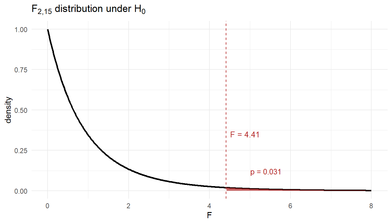
Since $p \approx 0.031 \le 0.05$ (equivalently $F = 4.41$ exceeds the critical value $F^* \approx 3.68$), reject $H_0$. At the 5% significance level there is sufficient evidence that mean fitness scores differ across the three programs.

Practice Problems

These supplement the TEE Review. Work them with only the SRC, your calculator, and R-lite. Answers are collapsed – check yourself before peeking.

Multiple Choice (Conceptual)

MC Problem 1 – Type II error

A Type II error occurs when:

We reject $H_0$ when $H_0$ is true
We fail to reject $H_0$ when $H_0$ is false
We reject $H_0$ when $H_a$ is true
The p-value is less than $\alpha$

Answer

(b) Type II = failing to reject a false $H_0$. Type I (a) is the opposite. Power = $1 - P(\text{Type II})$.

MC Problem 2 – Standard error of the mean

The standard error of $\bar{X}$ is:

$\sigma$
$\sigma^2 / n$
$\sigma / \sqrt{n}$
$s$

Answer

(c) $\sigma/\sqrt{n}$. Estimated by $s/\sqrt{n}$ when $\sigma$ is unknown.

MC Problem 3 – $R^2$ interpretation

A simple linear regression of $y$ on $x$ has $R^2 = 0.81$. The correct interpretation is:

81% of the values of $y$ equal $\hat{y}$
The correlation between $x$ and $y$ is 0.81
81% of the variability in $y$ is explained by the linear regression on $x$
The model predicts $y$ correctly 81% of the time

Answer

(c) $R^2$ is the proportion of variability in $y$ explained by the model. (The correlation $r = \pm 0.9$ here, not 0.81.)

MC Problem 4 – Mutually exclusive

If $A$ and $B$ are mutually exclusive with $P(A) > 0$ and $P(B) > 0$, then $A$ and $B$ are:

Independent
Dependent
Either independent or dependent depending on $P(A)$ and $P(B)$
Exhaustive

Answer

(b) Dependent. Mutually exclusive means $P(A \cap B) = 0$, but $P(A) P(B) > 0$, so $P(A \cap B) \ne P(A)P(B)$.

Event Probability

Problem EP-1 – Cadet club survey

A survey of 400 cadets finds 220 are in a club sport, 180 are in a tactical club, and 90 are in both.

$P$(at least one club)
$P$(neither)
$P$(only club sport, not tactical)

Answer

$\frac{220 + 180 - 90}{400} = \frac{310}{400} = 0.775$
$1 - 0.775 = 0.225$
$\frac{220 - 90}{400} = \frac{130}{400} = 0.325$

Problem EP-2 – Two dice

Roll two fair six-sided dice. Find:

$P$(sum equals 7)
$P$(sum is at least 10)
$P$(at least one die shows a 6)

Answer

$6/36 = 1/6 \approx 0.167$
Sums of 10, 11, 12: $\{(4,6),(5,5),(6,4),(5,6),(6,5),(6,6)\} = 6/36 = 1/6$
$P(\text{at least one 6}) = 1 - P(\text{no 6}) = 1 - (5/6)^2 = 11/36 \approx 0.306$

Conditional Probability and Bayes

Problem CP-1 – Maintenance flag

A motor pool’s preventive-maintenance scanner flags vehicles needing service. 8% of vehicles in the fleet actually need service. Among those that need service, the scanner flags 92% of the time. Among those that don’t need service, the scanner mistakenly flags 6% of the time.

What is the probability a randomly selected vehicle is flagged?
Given a vehicle is flagged, what is the probability it actually needs service?

Answer

Let $S$ = needs service, $F$ = flagged. $P(S) = 0.08$, $P(F|S) = 0.92$, $P(F|S^c) = 0.06$.

$P(F) = (0.92)(0.08) + (0.06)(0.92) = 0.0736 + 0.0552 = 0.1288$
$P(S|F) = \dfrac{(0.92)(0.08)}{0.1288} = \dfrac{0.0736}{0.1288} \approx 0.571$

So even with a flagged scan, only about 57% actually need service – because the base rate is low.

Problem CP-2 – Cards without replacement

Three cards are drawn without replacement from a standard 52-card deck.

$P$(all three are hearts)
$P$(at least one is a face card – J, Q, K)

Answer

$\dfrac{13}{52} \cdot \dfrac{12}{51} \cdot \dfrac{11}{50} = \dfrac{1716}{132600} \approx 0.0129$
$P(\text{none face}) = \dfrac{40}{52} \cdot \dfrac{39}{51} \cdot \dfrac{38}{50} \approx 0.4471$, so $P(\text{at least one}) \approx 0.553$

Binomial Distribution

Problem BIN-1 – APFT pass rate

Historically 85% of cadets pass the APFT on their first attempt. A platoon of 30 cadets takes the test. Let $X$ be the number who pass.

Identify the distribution of $X$.
$P(X = 28)$
$P(X \ge 25)$
$E[X]$ and $V[X]$

Answer

$X \sim \text{Bin}(n = 30,\, p = 0.85)$
$P(X = 28) = \binom{30}{28}(0.85)^{28}(0.15)^2$. R-lite: dbinom(28, 30, 0.85) $\approx 0.1234$
1 - pbinom(24, 30, 0.85) $\approx 0.9303$
$E[X] = 30 \cdot 0.85 = 25.5$, $V[X] = 30(0.85)(0.15) = 3.825$

Problem BIN-2 – Marksmanship qualification

A rifle marksman hits a target with probability 0.7 on each shot. She fires 12 shots independently.

Probability she hits exactly 9 shots.
Probability she hits between 7 and 10 shots, inclusive.
Probability she misses at most 2 shots.

Answer

$X \sim \text{Bin}(12, 0.7)$.

dbinom(9, 12, 0.7) $\approx 0.2397$
pbinom(10, 12, 0.7) - pbinom(6, 12, 0.7) $\approx 0.8367$
“At most 2 misses” = “at least 10 hits”: 1 - pbinom(9, 12, 0.7) $\approx 0.2528$

Poisson Distribution

Problem POIS-1 – Helpdesk calls

A help desk receives an average of 6 calls per hour, modeled as Poisson.

$P$(exactly 4 calls in an hour)
$P$(more than 8 calls in an hour)
$P$(exactly 12 calls in a 2-hour window)

Answer

$\lambda = 6$. dpois(4, 6) $\approx 0.1339$
1 - ppois(8, 6) $\approx 0.1528$
Over 2 hours, $\lambda = 12$. dpois(12, 12) $\approx 0.1144$

Problem POIS-2 – Defects per square meter

Manufacturing defects on a roll of fabric occur at an average rate of 0.4 defects per square meter, modeled as Poisson.

Probability a randomly chosen square meter has no defects.
Probability a 5 m$^2$ section has at least 3 defects.

Answer

$\lambda = 0.4$. $P(X = 0) = e^{-0.4} \approx 0.6703$
Over 5 m$^2$, $\lambda = 2$. 1 - ppois(2, 2) $\approx 0.3233$

Exponential Distribution

Problem EXP-1 – Time between radio messages

The time between radio messages on a tactical net is exponential with mean 7 minutes.

Probability the next message arrives within 5 minutes.
Probability more than 10 minutes pass with no message.
Median time between messages.

Answer

$\lambda = 1/7$ per minute.

$P(T \le 5) = 1 - e^{-5/7} \approx 0.5105$
$P(T > 10) = e^{-10/7} \approx 0.2397$
Median: $1 - e^{-\lambda t} = 0.5 \Rightarrow t = 7\ln 2 \approx 4.85$ min

Problem EXP-2 – Component lifetime

A radio component has lifetime exponential with mean 1,200 hours.

Probability a component lasts more than 2,000 hours.
The 10th-percentile lifetime (only 10% of components fail before this).
If a component has already lasted 1,500 hours, what is the probability it lasts at least another 1,200 hours?

Answer

$\mu = 1200$, $\lambda = 1/1200$.

$e^{-2000/1200} \approx 0.1889$
$1 - e^{-t/1200} = 0.10 \Rightarrow t = -1200 \ln(0.9) \approx 126.4$ hours
Memoryless property: $P(T > 2700 \mid T > 1500) = P(T > 1200) = e^{-1} \approx 0.3679$

Normal Distribution

Problem NORM-1 – Cadet height

Male cadet heights are approximately normal with $\mu = 70$ in and $\sigma = 2.8$ in.

Probability a randomly chosen male cadet is over 6 ft tall (72 in).
Probability his height is between 68 and 73 inches.
The 95th percentile of male cadet heights.

Answer

$z = (72 - 70)/2.8 = 0.714$. $P(Z > 0.714) \approx 0.2375$
$z_1 = (68-70)/2.8 = -0.714$, $z_2 = (73-70)/2.8 = 1.071$. $P \approx 0.8580 - 0.2375 = 0.6205$
$z = 1.645 \Rightarrow x = 70 + 1.645(2.8) \approx 74.6$ in

Problem NORM-2 – Battery life

Tactical radio battery life is approximately normal with $\mu = 18$ hr, $\sigma = 2.5$ hr.

Probability a battery lasts less than 14 hours.
Battery life $b$ such that 90% of batteries last at least $b$ hours.

Answer

$z = (14 - 18)/2.5 = -1.6$. $P(Z < -1.6) \approx 0.0548$
Want $P(X \ge b) = 0.90$, so $P(X < b) = 0.10$. $z = -1.282 \Rightarrow b = 18 - 1.282(2.5) \approx 14.8$ hr

One-Sample t-Test

Problem T1-1 – Land Nav completion time

The published Land Nav standard for a course is 120 minutes. A sample of $n = 16$ cadets has $\bar{x} = 128$ min and $s = 14$ min. Test at $\alpha = 0.05$ whether mean time differs from 120.

State $H_0$ and $H_a$.
Compute the test statistic and p-value.
Conclude in context.
95% CI for $\mu$.

Answer

$H_0: \mu = 120$, $H_a: \mu \ne 120$.
$t = \dfrac{128 - 120}{14/\sqrt{16}} = \dfrac{8}{3.5} \approx 2.286$ on 15 df. Two-sided p $\approx$ 2*pt(-2.286, 15) $\approx 0.0376$.
Reject $H_0$ at $\alpha = 0.05$. Evidence the mean Land Nav time differs from 120 min.
$128 \pm t_{0.025,15} \cdot 3.5 = 128 \pm 2.131 \cdot 3.5 = (120.5,\ 135.5)$ min

One-Proportion z-Test

Problem P1-1 – Tutoring program

A tutoring program claims more than 70% of attendees pass the next WPR. Of $n = 200$ attendees, 152 passed. Test at $\alpha = 0.05$.

State the hypotheses.
Test statistic and p-value.
Conclude.

Answer

$H_0: p = 0.70$, $H_a: p > 0.70$.
$\hat{p} = 152/200 = 0.76$. $z = \dfrac{0.76 - 0.70}{\sqrt{(0.70)(0.30)/200}} = \dfrac{0.06}{0.0324} \approx 1.852$. $p$-value $= P(Z > 1.852) \approx 0.0320$.
Reject $H_0$ at $\alpha = 0.05$. Evidence the pass rate exceeds 70%.

Two-Sample t-Test (Independent)

Problem T2-1 – Two ruck-march routes

Two ruck-march routes are compared. Route A: $n_1 = 18$, $\bar{x}_1 = 154$ min, $s_1 = 12$ min. Route B: $n_2 = 20$, $\bar{x}_2 = 161$ min, $s_2 = 14$ min. Test whether mean times differ at $\alpha = 0.05$ using conservative df.

Hypotheses.
Test statistic and p-value (use $\min(n_1-1, n_2-1) = 17$ df).
95% CI for $\mu_A - \mu_B$.

Answer

$H_0: \mu_A = \mu_B$, $H_a: \mu_A \ne \mu_B$.
SE $= \sqrt{12^2/18 + 14^2/20} = \sqrt{8 + 9.8} = \sqrt{17.8} \approx 4.219$. $t = (154 - 161)/4.219 \approx -1.659$ on 17 df. Two-sided p $\approx$ 2*pt(-1.659, 17) $\approx 0.115$.
$-7 \pm t_{0.025, 17}(4.219) = -7 \pm 2.110(4.219) = (-15.9,\ 1.9)$ min. CI includes 0 – consistent with failing to reject.

Paired t-Test

Problem PT-1 – Before/after PT score

Eight cadets take a 2-mile run before and after a 6-week conditioning program. Differences (before $-$ after, in seconds) for each cadet:

8, 12, 15, 4, 22, 9, 18, 6

Test at $\alpha = 0.05$ whether the program reduces run time (before $>$ after).

Answer

$\bar{d} = 11.75$, $s_d \approx 6.20$, $n = 8$.

$H_0: \mu_d = 0$, $H_a: \mu_d > 0$.

$t = \dfrac{11.75}{6.20/\sqrt{8}} = \dfrac{11.75}{2.193} \approx 5.36$ on 7 df. p-value $\approx 0.0005$. Reject $H_0$ – strong evidence the program reduces run time.

Two-Proportion z-Test

Problem P2-1 – Recruiting yield

Recruiting district A signs 84 of 300 contacted prospects; district B signs 72 of 320. Test whether signing rates differ at $\alpha = 0.05$.

Hypotheses.
Test statistic and p-value (use pooled SE).
95% CI for $p_A - p_B$ (use unpooled SE).

Answer

$\hat{p}_A = 0.28$, $\hat{p}_B = 0.225$. Pooled $\hat{p} = (84 + 72)/(300 + 320) = 156/620 = 0.2516$.

$H_0: p_A = p_B$; $H_a: p_A \ne p_B$.
Pooled SE $= \sqrt{0.2516(1 - 0.2516)(1/300 + 1/320)} \approx 0.0349$. $z = (0.28 - 0.225)/0.0349 \approx 1.576$. Two-sided p $\approx 0.115$. Fail to reject.
Unpooled SE $= \sqrt{0.28 \cdot 0.72/300 + 0.225 \cdot 0.775/320} \approx 0.0348$. CI: $0.055 \pm 1.96(0.0348) = (-0.013,\ 0.123)$. CI includes 0.

Simple Linear Regression

Problem SLR-1 – Study hours and exam score

A regression of exam score ($y$, out of 100) on weekly study hours ($x$) over $n = 28$ cadets gives $\hat{y} = 52 + 3.8 x$, $R^2 = 0.58$, slope p-value $< 0.001$. Data range: 1–14 hours/week.

Interpret the slope.
Interpret $R^2$.
Predict the exam score for a cadet who studies 7 hr/week.
Should you predict for a cadet who studies 25 hr/week? Why or why not?

Answer

For each additional hour of weekly study, predicted exam score increases by 3.8 points on average.
58% of variability in exam score is explained by the linear regression on weekly study hours.
$52 + 3.8(7) = 78.6$ points.
No – extrapolation. 25 hr/week is far outside the observed range (1–14). The linear pattern observed in the data may not hold there.

Multiple Linear Regression

Problem MLR-1 – Salary model

Predicting starting salary ($y$, in $1,000s) from years of experience ($x_1$), GPA ($x_2$), and an indicator for engineering major ($x_3 = 1$ if engineering, 0 otherwise):

\[\hat{y} = 32 + 1.6\,x_1 + 4.5\,x_2 + 8.2\,x_3\]

with adjusted $R^2 = 0.74$. All coefficients are statistically significant at $\alpha = 0.05$.

Interpret the coefficient on $x_1$.
Interpret the coefficient on $x_3$.
Predict starting salary for an engineering major with GPA 3.5 and 2 years of experience.

Answer

For each additional year of experience, predicted salary increases by $1,600 on average, holding GPA and major constant.
Engineering majors earn on average $8,200 more than non-engineering majors, holding experience and GPA constant.
$32 + 1.6(2) + 4.5(3.5) + 8.2(1) = 32 + 3.2 + 15.75 + 8.2 = 59.15$ → $59,150

Problem MLR-2 – Interpreting non-significance

In the same kind of model, suppose the coefficient on a fourth predictor (number of weekly hours worked) has p-value 0.42. What does this tell you?

Answer

After controlling for the other predictors in the model, there is no statistically significant evidence that weekly hours worked is linearly associated with salary. (Note: this does not mean hours don’t matter – only that, given the other predictors, the additional contribution is not significant.)

One-Way ANOVA

Problem ANOVA-1 – Three training programs

Three platoon-level training programs (A, B, C) are compared on a 100-point evaluation. ANOVA output:

            Df Sum Sq Mean Sq F value  Pr(>F)
program      2  840   420.0    7.78   0.0011
Residuals   42 2268    54.0

State $H_0$ and $H_a$.
Conclude at $\alpha = 0.05$.
What is the next step if you reject $H_0$?

Answer

$H_0: \mu_A = \mu_B = \mu_C$. $H_a:$ at least one mean differs.
Test statistic from the table: $F = 7.78$ on $(k-1,\,N-k) = (2,\,42)$ df.

p-value (right tail of the $F_{2,42}$ density):

1 - pf(7.78, df1 = 2, df2 = 42)
# [1] 0.001354

So $p \approx 0.0014$. Since $p \le 0.05$, reject $H_0$. At the 5% significance level, there is sufficient evidence that at least one program’s mean evaluation score differs from the others.

Run Tukey’s HSD to identify which pairs of means differ while controlling the family-wise error rate. ANOVA tells you that groups differ; Tukey tells you which.

Problem ANOVA-2 – Reading Tukey output

TukeyHSD output for the three programs above:

        diff    lwr    upr   p adj
B - A   8.20   1.10  15.30  0.020
C - A  10.50   3.40  17.60  0.002
C - B   2.30  -4.80   9.40  0.715

Which pairs of programs differ at the family-wise 5% level? Construct the letter/underline summary.

Answer

B vs. A ($p = 0.020$) and C vs. A ($p = 0.002$) differ. C vs. B does not ($p = 0.715$, CI includes 0).

Letters: A is its own group; B and C share a group. \[\bar{x}_A \qquad \underline{\bar{x}_B \quad \bar{x}_C}\]

Before You Leave

Today

TEE covers everything from L1–L37. Use the Review + Solutions + SRC to study.
Bring your SRC, calculator, and R-lite knowledge. Show up early.

Any questions? Office hours and email are open through the TEE.

Next Lesson

Lesson 40: Course Drop – Course Write-Up

Final Graded Event

TEE – 12, 13, 15 May 2026 (per section schedule above) – 300 points

	One-Sample Mean (Large)	One-Sample Mean (Small)	One Proportion	Two-Sample Mean (Large)	Two-Sample Mean (Small)	Paired Mean	Two Proportions	One-Way ANOVA
Parameter	\(\mu\)	\(\mu\)	\(p\)	\(\mu_1 - \mu_2\)	\(\mu_1 - \mu_2\)	\(\mu_d\)	\(p_1 - p_2\)	\(\mu_1, \dots, \mu_k\)
\(H_0\)	\(\mu = \mu_0\)	\(\mu = \mu_0\)	\(p = p_0\)	\(\mu_1 - \mu_2 = \Delta_0\)	\(\mu_1 - \mu_2 = \Delta_0\)	\(\mu_d = \Delta_0\)	\(p_1 - p_2 = 0\)	\(\mu_1 = \cdots = \mu_k\)
\(H_a\)	\(\mu \neq, <, > \mu_0\)	\(\mu \neq, <, > \mu_0\)	\(p \neq, <, > p_0\)	\(\mu_1 - \mu_2 \neq, <, > 0\)	\(\mu_1 - \mu_2 \neq, <, > 0\)	\(\mu_d \neq, <, > 0\)	\(p_1 - p_2 \neq, <, > 0\)	at least one \(\mu_i\) differs
Test Statistic	\(z = \dfrac{\bar{x} - \mu_0}{\sigma / \sqrt{n}}\)	\(t = \dfrac{\bar{x} - \mu_0}{s / \sqrt{n}}\)	\(z = \dfrac{\hat{p} - p_0}{\sqrt{p_0(1-p_0)/n}}\)	\(z = \dfrac{\bar{x}_1 - \bar{x}_2}{\sqrt{s_1^2/n_1 + s_2^2/n_2}}\)	\(t = \dfrac{\bar{x}_1 - \bar{x}_2}{\sqrt{s_1^2/n_1 + s_2^2/n_2}}\)	\(t = \dfrac{\bar{d} - \Delta_0}{s_d / \sqrt{n}}\)	\(z = \dfrac{\hat{p}_1 - \hat{p}_2}{\sqrt{\hat{p}(1-\hat{p})(1/n_1 + 1/n_2)}}\)	\(F = \dfrac{MSTr}{MSE}\)
Distribution	\(N(0,1)\)	\(t_{n-1}\)	\(N(0,1)\)	\(N(0,1)\)	\(t_{\min(n_1-1, n_2-1)}\)	\(t_{n-1}\)	\(N(0,1)\)	\(F_{k-1,\,N-k}\)
Left-tailed \(p\)	`pnorm(z)`	`pt(t, df)`	`pnorm(z)`	`pnorm(z)`	`pt(t, df)`	`pt(t, df)`	`pnorm(z)`	–
Right-tailed \(p\)	`1 - pnorm(z)`	`1 - pt(t, df)`	`1 - pnorm(z)`	`1 - pnorm(z)`	`1 - pt(t, df)`	`1 - pt(t, df)`	`1 - pnorm(z)`	`1 - pf(F, df1, df2)`
Two-tailed \(p\)	`2*(1 - pnorm(abs(z)))`	`2*(1 - pt(abs(t), df))`	`2*(1 - pnorm(abs(z)))`	`2*(1 - pnorm(abs(z)))`	`2*(1 - pt(abs(t), df))`	`2*(1 - pt(abs(t), df))`	`2*(1 - pnorm(abs(z)))`	–
Conditions	\(n \geq 30\)	Normal pop or \(n \geq 30\)	\(np_0 \geq 10\) & \(n(1-p_0) \geq 10\)	\(n_1, n_2 \geq 30\)	Both pops \(\sim\) Normal	Diffs \(\sim\) Normal or \(n \geq 30\)	\(n_i\hat{p}_i \geq 10\) & \(n_i(1-\hat{p}_i) \geq 10\)	Indep. samples; equal-variance, approx. normal within groups

	One-Sample Mean (Large)	One-Sample Mean (Small)	One Proportion	Two-Sample Mean	Paired Mean	Two Proportions
Parameter	\(\mu\)	\(\mu\)	\(p\)	\(\mu_1 - \mu_2\)	\(\mu_d\)	\(p_1 - p_2\)
Formula	\(\bar{x} \pm z_{\alpha/2} \cdot \dfrac{\sigma}{\sqrt{n}}\)	\(\bar{x} \pm t_{\alpha/2,\, n-1} \cdot \dfrac{s}{\sqrt{n}}\)	\(\hat{p} \pm z_{\alpha/2} \cdot \sqrt{\dfrac{\hat{p}(1-\hat{p})}{n}}\)	\((\bar{x}_1 - \bar{x}_2) \pm t_{\alpha/2} \cdot \sqrt{\dfrac{s_1^2}{n_1} + \dfrac{s_2^2}{n_2}}\)	\(\bar{d} \pm t_{\alpha/2,\, n-1} \cdot \dfrac{s_d}{\sqrt{n}}\)	\((\hat{p}_1 - \hat{p}_2) \pm z_{\alpha/2} \cdot \sqrt{\dfrac{\hat{p}_1(1-\hat{p}_1)}{n_1} + \dfrac{\hat{p}_2(1-\hat{p}_2)}{n_2}}\)
Conditions	\(n \geq 30\)	Normal pop or \(n \geq 30\)	\(n\hat{p} \geq 10\) & \(n(1-\hat{p}) \geq 10\)	\(n_1, n_2 \geq 30\) (or Normal pops)	Diffs \(\sim\) Normal or \(n \geq 30\)	\(n_i\hat{p}_i \geq 10\) & \(n_i(1-\hat{p}_i) \geq 10\)

Lesson 39: TEE Review

TEE Logistics

TEE Review Materials

Course Outline – Everything We Did

Block I: Data and Randomness (Lessons 1–16)

Block II: Inference (Lessons 17–27)

Block III: Regression and ANOVA (Lessons 28–38)

Reference Tables

Named Distributions

Summary of Hypothesis Tests

Summary of Confidence Intervals

Possible Pitfalls

Break!

Reese

Cal

Worked Examples

Bayes’ Theorem – The Eyewitness Cab Problem

Exponential and Poisson – Tactical Radio Net

One-Way ANOVA – Comparing three training programs

Practice Problems

Multiple Choice (Conceptual)

Event Probability

Conditional Probability and Bayes

Binomial Distribution

Poisson Distribution

Exponential Distribution

Normal Distribution

One-Sample t-Test

One-Proportion z-Test

Two-Sample t-Test (Independent)

Paired t-Test

Two-Proportion z-Test

Simple Linear Regression

Multiple Linear Regression

One-Way ANOVA

Before You Leave

Today

Next Lesson

Final Graded Event

In Memory of Travis Clonch