Lesson 25: Paired t-Test

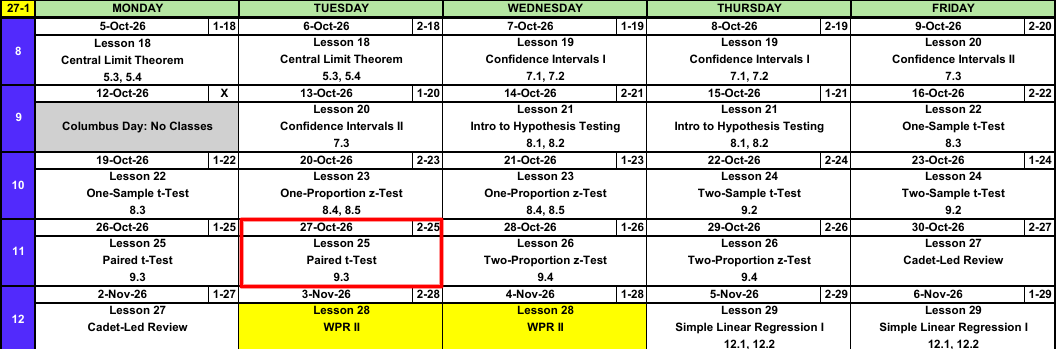
Calendar

Break!

MAJ Lovas, time to talk about your family!

Warm-Up

IOCT: Two Sections

Does Military Movement lower IOCT times? One section ran the IOCT after finishing Military Movement. A different section ran it before starting. Treat each section as a random sample. Test at \(\alpha = 0.05\).

Group	\(n\)	\(\bar{x}\) (min)	\(s\) (min)
1: After	13	3.81	0.41
2: Before	12	4.02	0.38

Answer

1. Hypotheses: \(H_0: \mu_1 - \mu_2 = 0\) versus \(H_a: \mu_1 - \mu_2 < 0\). \(\mu_1\) and \(\mu_2\) are the true mean IOCT times of all cadets after and before Military Movement. Lower times for group 1 means \(< 0\).

2. Conditions: Two independent random samples. Both \(n \le 40\), so both populations approximately normal.

3. Test statistic:

\[t = \frac{3.81 - 4.02}{\sqrt{\dfrac{0.41^2}{13} + \dfrac{0.38^2}{12}}} = \frac{-0.21}{0.1580} = \mathbf{-1.33}\]

\[\nu = \frac{\left(0.0129 + 0.0120\right)^2}{\dfrac{0.0129^2}{12} + \dfrac{0.0120^2}{11}} = 23.00, \text{ round down to } \mathbf{22}\]

4. P-value: \(P(T \le -1.33) = \mathbf{0.0987}\). pt(-1.329, 22)

5. Decision: \(0.0987 > 0.05\). Fail to reject \(H_0\).

6. Conclusion: At the 5% level there is insufficient evidence that the true mean IOCT time of cadets is lower after Military Movement than before.

IOCT: Same Cadets

Now change the design. Ten randomly selected cadets ran the IOCT before Military Movement, then the same ten ran it again after.

Cadet	1	2	3	4	5	6	7	8	9	10
Before	4.32	3.75	4.67	3.58	4.21	3.62	4.55	3.44	4.05	4.48
After	4.10	3.61	4.38	3.47	3.89	3.50	4.22	3.36	3.79	4.31

Can we run the same test as above?

Answer

We could, but we can be more accurate. Each before time is linked to an after time from the same cadet, and a fast cadet is fast both times. That is paired data. Subtract within each cadet and the ten differences are one sample, so we run the Lesson 22 one-sample \(t\) test on them. See The Steps below.

What We Did: Lessons 18 to 24

Review: Central Limit Theorem (Lesson 18)

\(\bar{X} \sim N\left(\mu,\ \left(\dfrac{\sigma}{\sqrt{n}}\right)^2\right)\), approximately, for \(n > 40\)
Normal population: exact for any \(n\)
pnorm(x, mu, sigma/sqrt(n))
\(\hat{p} \sim N\left(p,\ \dfrac{p(1-p)}{n}\right)\), approximately, when \(np \ge 10\) and \(n(1-p) \ge 10\)

Review: Confidence Intervals I (Lesson 19)

\(\text{estimate} \pm \text{critical value} \times \text{standard error}\)
Mean, \(n > 40\): \(\bar{x} \pm z_{\alpha/2}\,\dfrac{s}{\sqrt{n}}\)
Proportion, \(n\hat{p} \ge 10\) and \(n(1-\hat{p}) \ge 10\): \(\hat{p} \pm z_{\alpha/2}\sqrt{\dfrac{\hat{p}(1-\hat{p})}{n}}\)
qnorm(0.975) for 95%, qnorm(0.95) for 90%, qnorm(0.995) for 99%
95% confident describes the method

Review: Confidence Intervals II (Lesson 20)

Small sample, normal population: \(\bar{x} \pm t_{\alpha/2,\,n-1}\,\dfrac{s}{\sqrt{n}}\)
\(\text{df} = n - 1\), qt(0.975, n - 1) for 95%
\(t_{\alpha/2,\,n-1} > z_{\alpha/2}\), so the \(t\) interval is wider
Sample size for width \(w\): \(n = \left(\dfrac{2\,z_{\alpha/2}\,\sigma}{w}\right)^2\), rounded up

Review: Intro to Hypothesis Testing (Lesson 21)

\(H_0: \mu = \mu_0\) versus \(H_a\): \(\mu < \mu_0\), \(\mu > \mu_0\), or \(\mu \ne \mu_0\)
\(z = \dfrac{\bar{x} - \mu_0}{s/\sqrt{n}}\), random sample, \(n > 40\)
P-value: pnorm(z), 1 - pnorm(z), 2 * pnorm(-abs(z))
Reject \(H_0\) if the P-value is at or below \(\alpha\), otherwise fail to reject
Type I: reject a true \(H_0\) (\(\alpha\)). Type II: fail to reject a false \(H_0\) (\(\beta\))
Fail to reject is not accept

Review: One-Sample t-Test (Lesson 22)

\(t = \dfrac{\bar{x} - \mu_0}{s/\sqrt{n}}\), \(\text{df} = n - 1\)
Random sample, \(n \le 40\), population approximately normal
P-value: pt(t, n - 1), 1 - pt(t, n - 1), 2 * pt(-abs(t), n - 1)
t.test(x, mu = mu0, alternative = "two.sided")

Review: One-Proportion z-Test (Lesson 23)

\(z = \dfrac{\hat{p} - p_0}{\sqrt{p_0(1 - p_0)/n}}\)
Random sample, \(np_0 \ge 10\) and \(n(1 - p_0) \ge 10\)
The test uses \(p_0\), the interval uses \(\hat{p}\)
Statistically significant does not mean practically significant

Review: Two-Sample t-Test (Lesson 24)

\(t = \dfrac{(\bar{x}_1 - \bar{x}_2) - \Delta_0}{\sqrt{s_1^2/n_1 + s_2^2/n_2}}\), approximate df \(\nu\), rounded down
Two independent random samples, both populations approximately normal (or both \(n > 40\))
Interval: \((\bar{x}_1 - \bar{x}_2) \pm t_{\alpha/2,\,\nu}\sqrt{s_1^2/n_1 + s_2^2/n_2}\)
Name group 1 first, then put the claim in \(H_a\)
t.test(x1, x2, alternative = "greater")

What We’re Doing: Lesson 25

Objectives

Identify paired data and the appropriate paired design. (SLO 3)
State and check the assumptions of the paired \(t\) test. (SLO 5)
Carry out the paired \(t\) test for a mean difference. (SLO 5)
Construct and interpret a confidence interval for a mean difference. (SLO 5)
Explain how pairing reduces the standard error relative to an independent two-sample analysis. (SLO 3, 5)

Required Reading

Devore 9.3

The Takeaway for Today

Key Concepts from Lesson 25

Paired data: two measurements on the same unit (or matched units). Analyze the differences \(d_i = x_i - y_i\).
Test statistic: \(t = \dfrac{\bar{d} - \Delta_0}{s_D/\sqrt{n}}\), \(\text{df} = n - 1\)
Conditions: random sample of pairs, differences approximately normal (or \(n > 40\))
Interval: \(\bar{d} \pm t_{\alpha/2,\,n-1}\dfrac{s_D}{\sqrt{n}}\)
Why pair: pairing removes the unit to unit variability, so \(s_D/\sqrt{n}\) is much smaller than the two-sample standard error

Paired Data

Paired Design

Each observation in one sample is linked to exactly one observation in the other: same cadet twice, twins, left and right hand, same squad under two conditions.
\(n\) pairs, so \(n_1 = n_2 = n\).
The two measurements on a unit are not independent. A fast cadet is fast before and after Military Movement. The L24 test still runs, but it ignores the pairing.
Fix: subtract within each pair. The differences \(d_1, \dots, d_n\) are one sample, and we already know how to test one sample (Lesson 22).

Paired or independent?

Pulse of \(15\) cadets before and after a ruck march.
Sleep hours of \(20\) cadets in Eisenhower Barracks and \(20\) cadets in Lee Barracks.
\(14\) cadets each run the IOCT once in new shoes and once in old shoes, order randomized.
WPR I and WPR II scores for every cadet in one section.

Answer

Paired. Same cadets twice.
Independent. Two separate groups. Equal sample sizes do not make it paired.
Paired. Each cadet runs both conditions.
Paired. Two scores on each cadet.

Paired \(t\) Test

Paired \(t\) Test for \(\mu_D\)

With \(D = X - Y\) for each pair, \(\mu_D = \mu_1 - \mu_2\).

\[\bar{d} = \frac{1}{n}\sum d_i, \qquad s_D = \sqrt{\frac{\sum (d_i - \bar{d})^2}{n - 1}}\]

\[t = \frac{\bar{d} - \Delta_0}{s_D/\sqrt{n}}, \qquad \text{df} = n - 1\]

Hypotheses: \(H_0: \mu_D = \Delta_0\) versus \(H_a\): \(\mu_D > \Delta_0\), \(< \Delta_0\), or \(\ne \Delta_0\). Usually \(\Delta_0 = 0\).
Conditions: random sample of pairs; the differences are approximately normal, or \(n > 40\). Check with a histogram or normal probability plot of the \(d_i\), not of the two samples.
If \(H_0\) is true, \(T \sim t_{n-1}\)

\(H_a\)	P-value
\(\mu_D > \Delta_0\)	`1 - pt(t, n - 1)`
\(\mu_D < \Delta_0\)	`pt(t, n - 1)`
\(\mu_D \ne \Delta_0\)	`2 * pt(-abs(t), n - 1)`

Confidence Interval for \(\mu_D\)

\[\bar{d} \pm t_{\alpha/2,\,n-1}\frac{s_D}{\sqrt{n}}\]

Same conditions as the test
Interval contains \(0\): no evidence of a difference. All positive: \(\mu_D > 0\). All negative: \(\mu_D < 0\).

Order of Subtraction

Define \(D\) before writing \(H_a\). “Faster after” with \(D = \text{after} - \text{before}\) is \(H_a: \mu_D < 0\). With \(D = \text{before} - \text{after}\) it is \(H_a: \mu_D > 0\). Same claim, sign flipped, same as L24.

The Steps

IOCT: Same Cadets

Back to the Warm-Up’s ten cadets. Does Military Movement lower IOCT times? Test at \(\alpha = 0.05\).

A Paired \(t\) Test Is a One-Sample \(t\) Test

Compute \(d_i = \text{after} - \text{before}\) for each cadet. Forget the two columns. The ten \(d_i\) are one sample, and we test \(H_0: \mu_D = 0\) exactly as in Lesson 22:

\[\text{Lesson 22: } t = \frac{\bar{x} - \mu_0}{s/\sqrt{n}} \qquad \longrightarrow \qquad \text{Today: } t = \frac{\bar{d} - 0}{s_D/\sqrt{n}}, \quad \text{df} = n - 1\]

Cadet	1	2	3	4	5	6	7	8	9	10
Before	4.32	3.75	4.67	3.58	4.21	3.62	4.55	3.44	4.05	4.48
After	4.10	3.61	4.38	3.47	3.89	3.50	4.22	3.36	3.79	4.31
\(d\) = After \(-\) Before	-0.22	-0.14	-0.29	-0.11	-0.32	-0.12	-0.33	-0.08	-0.26	-0.17

1. Hypotheses: State \(H_0\) and \(H_a\).

Answer

\[H_0: \mu_D = 0\]

\[H_a: \mu_D < 0\]

\(\mu_D\) is the true mean change in IOCT time (after minus before Military Movement) for all cadets. Faster after means a negative difference.

2. Conditions: What conditions allow us to do this?

Answer

Paired: the same cadets measured twice. Random sample of cadets. \(n = 10 \le 40\), so the differences must be approximately normal. Check with a histogram or normal probability plot of the ten \(d_i\).

3. Test statistic: Compute \(\bar{d}\), \(s_D\), and \(t\).

Answer

The mean and standard deviation of the \(d\) row, the same as \(\bar{x}\) and \(s\) for any one sample:

\[\bar{d} = -0.204, \qquad s_D = 0.0923\]

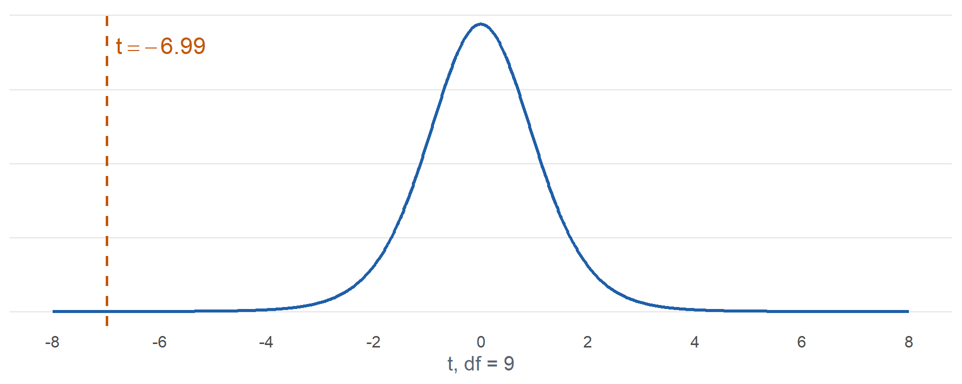
\[t = \frac{-0.204 - 0}{0.0923/\sqrt{10}} = \frac{-0.204}{0.0292} = \mathbf{-6.99}, \qquad \text{df} = 9\]

4. P-value: Find it.

Answer

t curve with 9 degrees of freedom. The test statistic is marked far in the left tail, beyond the visible area of the curve.

\[P(T \le -6.99) = \mathbf{0.000032}\]

pt(-6.991, 9)

5. Decision: Reject or fail to reject?

Answer

\(0.000032 \le 0.05\). Reject \(H_0\).

6. Conclusion: State it in context.

Answer

Since the P-value \(0.000032 \le \alpha = 0.05\), reject \(H_0\). At the 5% level there is sufficient evidence that the true mean IOCT time of cadets is lower after Military Movement than before.

Confidence interval: Build a 95% interval for \(\mu_D\) and interpret it.

Answer

\(t_{0.025,\,9} = 2.262\). qt(0.975, 9)

\[-0.204 \pm 2.262(0.0292) = (-0.270,\ -0.138)\]

We are 95% confident that Military Movement lowers the true mean IOCT time by between 0.138 and 0.270 minutes (about 8 to 16 seconds). All negative, consistent with rejecting \(H_0\).

Why Pair?

Two sections in the Warm-Up: fail to reject. Same cadets twice: reject, with a P-value near zero.

What if we ignored the pairing and ran the L24 two-sample test on the before and after columns?

Answer

	Paired	Two-sample (ignores pairing)
Estimate	\(\bar{d} = -0.204\)	\(\bar{x}_1 - \bar{x}_2 = -0.204\)
Standard error	\(s_D/\sqrt{n} = 0.0292\)	\(\sqrt{s_1^2/n_1 + s_2^2/n_2} = 0.1839\)
\(t\)	-6.99	-1.11
P-value	0.000032	0.1413
Decision	Reject \(H_0\)	Fail to reject \(H_0\)

Same estimate, very different standard error. Before times range from 3.44 to 4.67 minutes, and the two-sample standard error carries all of that cadet to cadet spread (\(s_1 \approx s_2 \approx 0.45\)). Subtracting within each cadet cancels it: the differences only vary by about \(s_D = 0.09\).

Pairing Reduces the Standard Error

Each difference removes what is constant about that unit (fitness, ability, body size).
Less variability in the \(d_i\), smaller \(s_D/\sqrt{n}\), larger \(|t|\), smaller P-value.
Paired data analyzed as two samples: the test still runs, but the larger standard error can hide a real effect.

In R

Twelve randomly selected cadets ran the 2 mile before and after a six week running program (minutes). Did the program lower run times?


    Paired t-test

data:  post and pre
t = -6.2678, df = 11, p-value = 3.053e-05
alternative hypothesis: true mean difference is less than 0
95 percent confidence interval:
      -Inf -0.356738
sample estimates:
mean difference 
           -0.5

paired = TRUE makes \(d_i\) = first vector minus second vector, here post minus pre
“Lower times” with \(D = \text{post} - \text{pre}\) means \(H_a: \mu_D < 0\), so alternative = "less"
Same output: t.test(post - pre, mu = 0, alternative = "less"), the one-sample test from L22 on the differences

What do you conclude at \(\alpha = 0.10\)?

Answer

\(\bar{d} = -0.50\) minutes, \(t = -6.27\), df \(= 11\), P-value \(= 0.000031 \le 0.10\). Reject \(H_0\).

At the 10% level there is sufficient evidence that the true mean 2 mile time of cadets is lower after the program than before it.

Inference Procedures

Parameter	Conditions	Test statistic	Confidence interval	Critical value	P-value by \(H_a\)
\(\mu\) \(\sigma\) known, or \(\sigma\) unknown and \(n > 40\)	Random sample \(\sigma\) known and population normal, or \(n > 40\)	\(z = \dfrac{\bar{x} - \mu_0}{\sigma/\sqrt{n}}\) use \(s\) for \(\sigma\) when \(n > 40\)	\(\bar{x} \pm z_{\alpha/2}\dfrac{\sigma}{\sqrt{n}}\)	`qnorm(1-a/2)`	\(>\) `1-pnorm(z)` \(<\) `pnorm(z)` \(\ne\) `2*pnorm(-abs(z))`
\(\mu\) \(\sigma\) unknown, \(n \le 40\)	Random sample Population approx. normal	\(t = \dfrac{\bar{x} - \mu_0}{s/\sqrt{n}} \sim t_{n-1}\)	\(\bar{x} \pm t_{\alpha/2,\,n-1}\dfrac{s}{\sqrt{n}}\)	`qt(1-a/2,n-1)`	\(>\) `1-pt(t,n-1)` \(<\) `pt(t,n-1)` \(\ne\) `2*pt(-abs(t),n-1)`
\(p\)	Random sample \(np_0 \ge 10\) \(n(1-p_0) \ge 10\)	\(z = \dfrac{\hat{p} - p_0}{\sqrt{p_0(1-p_0)/n}}\) the test uses \(p_0\)	\(\hat{p} \pm z_{\alpha/2}\sqrt{\dfrac{\hat{p}(1-\hat{p})}{n}}\) the interval uses \(\hat{p}\)	`qnorm(1-a/2)`	\(>\) `1-pnorm(z)` \(<\) `pnorm(z)` \(\ne\) `2*pnorm(-abs(z))`
\(\mu_1 - \mu_2\) independent	Two independent samples Both normal, or both \(n > 40\)	\(t = \dfrac{(\bar{x}_1 - \bar{x}_2) - \Delta_0}{\sqrt{s_1^2/n_1 + s_2^2/n_2}} \sim t_{\nu}\)	\((\bar{x}_1 - \bar{x}_2) \pm t_{\alpha/2,\,\nu}\sqrt{\dfrac{s_1^2}{n_1}+\dfrac{s_2^2}{n_2}}\)	`qt(1-a/2,nu)`	\(>\) `1-pt(t,nu)` \(<\) `pt(t,nu)` \(\ne\) `2*pt(-abs(t),nu)`
\(\mu_D\) paired	Random sample of pairs Differences approx. normal, or \(n > 40\)	\(t = \dfrac{\bar{d} - \Delta_0}{s_D/\sqrt{n}} \sim t_{n-1}\)	\(\bar{d} \pm t_{\alpha/2,\,n-1}\dfrac{s_D}{\sqrt{n}}\)	`qt(1-a/2,n-1)`	\(>\) `1-pt(t,n-1)` \(<\) `pt(t,n-1)` \(\ne\) `2*pt(-abs(t),n-1)`
\(p_1 - p_2\)

Board Problems

Problem 1: Paired or Independent?

Questions

For each, choose the test: paired \(t\) or two-sample \(t\).

Pushups of \(16\) cadets before and after a four week calisthenics plan.
Run times of a random sample of \(25\) cadets from Company A and \(25\) from Company B.
\(12\) squads each run a land nav course with paper maps and, a week later, with a GPS. Score is the squad’s total points found.
Weights of \(30\) cadets on the Arvin Gym scale and on the Keller clinic scale, to compare the scales.

Answers

Paired. Same cadets twice.
Two-sample. Two separate groups. Equal \(n\) does not make it paired.
Paired. The squad is the unit, measured under both conditions.
Paired. Each cadet stands on both scales.

Problem 2: Grip Strength

Eight randomly selected cadets had grip strength (kg) measured in the dominant and non-dominant hand. Is there a difference? Test at \(\alpha = 0.10\).

Cadet	1	2	3	4	5	6	7	8
Dominant	52	47	58	44	50	61	49	55
Non-dominant	48	46	53	45	47	56	46	51

Questions

Define \(D\) and state the hypotheses.
State the conditions.
Compute the differences, \(\bar{d}\), \(s_D\), and \(t\).
Find the P-value.
Decide and conclude.
Build and interpret a 90% interval for \(\mu_D\).

Answers

\(D\) = dominant \(-\) non-dominant.

\[H_0: \mu_D = 0\]

\[H_a: \mu_D \ne 0\]

\(\mu_D\) is the true mean difference in grip strength (dominant minus non-dominant) for all cadets.

Paired, random sample of cadets. \(n = 8 \le 40\), so the differences must be approximately normal.
\(d\) = 4, 1, 5, -1, 3, 5, 3, 4.

\[\bar{d} = 3.00, \qquad s_D = 2.070, \qquad t = \frac{3.00}{2.070/\sqrt{8}} = \mathbf{4.10}, \qquad \text{df} = 7\]

\[2P(T \ge 4.10) = \mathbf{0.0046}\]

2 * pt(-abs(4.099), 7)

Since the P-value \(0.0046 \le \alpha = 0.10\), reject \(H_0\). At the 10% level there is sufficient evidence that the true mean grip strength of cadets differs between the dominant and non-dominant hand.
\(t_{0.05,\,7} = 1.895\). qt(0.95, 7)

\[3.00 \pm 1.895(0.732) = (1.61,\ 4.39)\]

We are 90% confident that the dominant hand is, on average, between 1.61 and 4.39 kg stronger than the non-dominant hand.

Problem 3: Read the Output

Ten randomly selected cadets did 2 minutes of pushups at 0630 (am) and again at 1600 (pm) on the same day.


    Paired t-test

data:  pm and am
t = 6.8214, df = 9, p-value = 7.717e-05
alternative hypothesis: true mean difference is not equal to 0
95 percent confidence interval:
 1.804612 3.595388
sample estimates:
mean difference 
            2.7

Questions

How is \(D\) defined? What are \(H_0\) and \(H_a\)?
Report \(\bar{d}\), \(t\), df, and the P-value.
Decide at \(\alpha = 0.05\) and conclude in context.
Interpret the confidence interval.
Why does a paired test analyze the differences instead of the two columns?

Answers

\(D\) = pm \(-\) am (first vector minus second). \(H_0: \mu_D = 0\) versus \(H_a: \mu_D \ne 0\), from “true mean difference is not equal to 0.”
\(\bar{d} = 2.70\), \(t = 6.82\), df \(= 9\), P-value \(= 0.000077\).
\(0.000077 \le 0.05\). Reject \(H_0\). At the 5% level there is sufficient evidence that the true mean number of pushups differs between morning and afternoon.
We are 95% confident that cadets do, on average, between 1.80 and 3.60 more pushups in the afternoon than in the morning.
The morning and afternoon counts come from the same cadet, so they are not independent. A strong cadet is strong at both times. Each difference is one number per cadet, and the differences are a single random sample.

Problem 4: Ignore the Pairing

A classmate ran the same pushup data through the L24 test.


    Welch Two Sample t-test

data:  pm and am
t = 1.2557, df = 17.998, p-value = 0.2253
alternative hypothesis: true difference in means is not equal to 0
95 percent confidence interval:
 -1.817418  7.217418
sample estimates:
mean of x mean of y 
     45.7      43.0

Questions

What does this output conclude at \(\alpha = 0.05\)?
Both tests estimate the same difference. Why is this P-value so much larger?
Which test should we report, and why?

Answers

P-value \(= 0.2253 > 0.05\). Fail to reject \(H_0\): no evidence of a difference.
Same estimate, \(45.70 - 43.00 = 2.70\). The two-sample standard error includes the cadet to cadet spread (36 to 52 pushups). The paired standard error only includes how much each cadet’s change varies, which is much smaller. Smaller SE, larger \(|t|\), smaller P-value.
The paired test (Problem 3). Both tests run, but the paired test removes the cadet to cadet spread, so it is more accurate and detects the difference.

Before You Leave

Today

Paired data: two measurements on the same unit. Analyze \(d_i\).
\(t = \dfrac{\bar{d} - \Delta_0}{s_D/\sqrt{n}}\), \(\text{df} = n - 1\)
Interval: \(\bar{d} \pm t_{\alpha/2,\,n-1}\dfrac{s_D}{\sqrt{n}}\)
Define \(D\) first, then put the claim in \(H_a\)
Pairing removes unit to unit variability, so the standard error shrinks
t.test(x, y, paired = TRUE, alternative = "greater")

Any questions?

Next Lesson

Lesson 26: Two-Proportion z-Test

Check the large-sample conditions for inferences about \(p_1 - p_2\)
Carry out a large-sample \(z\) test for a difference between two population proportions
Construct and interpret a confidence interval for \(p_1 - p_2\)

Reading: Devore 9.4

Upcoming Graded Events

WebAssign 9.3: due at the start of Lesson 26
WPR II: Lesson 28 (covers Lessons 18-26)
TEE: 15-18 Dec 2026