Lesson 14: Exploratory Data Analysis (EDA)

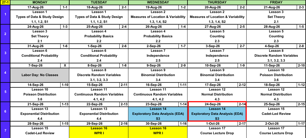
Calendar

---

Admin

WPR I Is Two Lessons Away

• Lesson 15 (25, 28 Sep) is the cadet-led review. Bring questions, not blank paper.
• Lesson 16 (29-30 Sep) is WPR I, covering Lessons 1 through 13.
• WPR I Review and Solutions

---

What We Did: Lessons 1 through 13

NoteReview: Data, Study Design, and Summaries (Lessons 1 and 2)

• Population vs sample, parameter (\(\mu\), \(\sigma\), \(p\)) vs statistic (\(\bar{x}\), \(s\), \(\hat{p}\)).
• Random sampling buys generalization, random assignment buys causation.
• Center: mean, median, trimmed mean. Spread: \(s^2\), \(s\), and the fourth spread \(f_s\).

NoteReview: Set Theory and Probability Basics (Lessons 3 and 4)

• Experiment, sample space \(\mathcal{S}\), event as a subset of \(\mathcal{S}\).
• Union is “or”, intersection is “and”, complement is “not”.
• Three axioms, the complement rule \(P(A') = 1 - P(A)\), and the addition rule \(P(A \cup B) = P(A) + P(B) - P(A \cap B)\).
• Equally likely outcomes: \(P(A) = N(A)/N\).

NoteReview: Counting (Lesson 5)

• Product rule: \(n_1 n_2 \cdots n_k\).
• Permutation (order matters): \(P_{k,n} = \dfrac{n!}{(n-k)!}\).
• Combination (order does not): \(\dbinom{n}{k} = \dfrac{n!}{k!\,(n-k)!}\).

NoteReview: Conditional Probability and Independence (Lessons 6 and 7)

• Conditional probability: \(P(A \mid B) = \dfrac{P(A \cap B)}{P(B)}\).
• Multiplication rule, Law of Total Probability, and Bayes’ Theorem.
• Independent: \(P(A \mid B) = P(A)\), tested with \(P(A \cap B) = P(A)\,P(B)\).
• \(P(\text{at least one}) = 1 - P(\text{none})\).

NoteReview: Discrete Random Variables (Lessons 8, 9, and 10)

• pmf: \(p_X(x) = P(X = x)\). cdf: \(F_X(x) = P(X \le x)\), a step function.
• Binomial: BINS, \(p(x) = \dbinom{n}{x} p^x (1-p)^{n-x}\), \(E(X) = np\), \(V(X) = np(1-p)\).
• Poisson: a rate and a window, \(p(x; \mu) = \dfrac{e^{-\mu}\mu^x}{x!}\), \(E(X) = V(X) = \mu\).
• \(E(X) = \sum_x x\,p_X(x)\) and \(V(X) = E(X^2) - [E(X)]^2\).

NoteReview: Continuous Random Variables (Lesson 11)

• Probability is area under the pdf: \(P(a \le X \le b) = \int_a^b f(x)\,dx\).
• \(P(X = c) = 0\), so \(\le\) and \(<\) give the same answer.
• cdf: \(F(x) = P(X \le x)\), and \(P(a \le X \le b) = F(b) - F(a)\).
• Percentile: solve \(F(c) = P(X \le c) = p\) for \(c\).
• \(E(X) = \int x\,f(x)\,dx\) and \(V(X) = E(X^2) - [E(X)]^2\).

NoteReview: Normal Distribution (Lesson 12)

• \(X \sim N(\mu, \sigma^2)\), with \(E(X) = \mu\) and \(V(X) = \sigma^2\).
• pnorm(x, mean, sd) is the cdf \(F(x) = P(X \le x)\). qnorm runs it backwards.
• Standardize with \(z = \dfrac{x - \mu}{\sigma}\) to land on \(Z \sim N(0, 1)\).
• Empirical rule: 68%, 95%, 99.7% within 1, 2, 3 standard deviations.
• \(z_\alpha\) has area \(\alpha\) to its right.

NoteReview: Exponential Distribution (Lesson 13)

• \(X \sim \text{Exp}(\lambda)\) models a wait, with \(E(X) = \sigma = 1/\lambda\).
• \(F(x) = P(X \le x) = 1 - e^{-\lambda x}\), so \(P(X > x) = e^{-\lambda x}\).
• pexp(x, rate) takes the rate, not the mean. qexp runs it backwards.
• Memoryless: time already waited does not change what comes next.
• Poisson counts events at rate \(\lambda\). The waits between them are \(\text{Exp}(\lambda)\).

---

Warm-Up: Count or Wait?

Walk-ins arrive at sick call at a rate of 4 per hour.

For each question: count or wait? Fully specify, then compute.

a) What is the probability exactly 2 cadets walk in during the next hour?

TipAnswer

A count.

\[Y \sim \text{Pois}(\mu = 4)\]

• Designate the random variable. \(Y\) is the number of walk-ins in the next hour.
• Name the distribution. Poisson.
• Specify the parameter. \(\mu = 4\) walk-ins.

\[P(Y = 2) = \frac{e^{-4} 4^2}{2!} = \mathbf{0.1465}\]

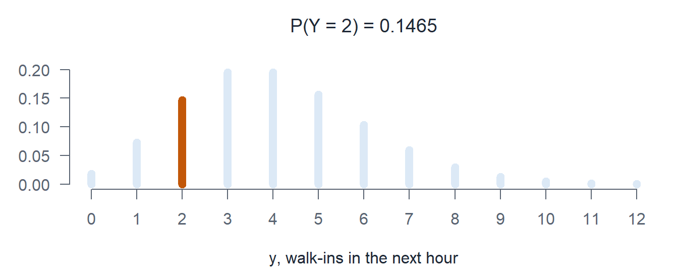
dpois(2, 4) = 0.1465

b) What is the probability the next cadet walks in within half an hour?

TipAnswer

A wait. Half an hour is \(x = 0.5\).

\[X \sim \text{Exp}(\lambda = 4)\]

• Designate the random variable. \(X\) is the hours until the next walk-in.
• Name the distribution. Exponential.
• Specify the parameter. \(\lambda = 4\) per hour.

\[P(X < 0.5) = 1 - e^{-4(0.5)} = 1 - e^{-2} = \mathbf{0.8647}\]

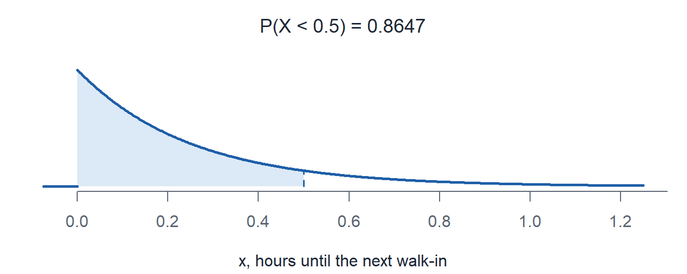
pexp(0.5, 4) = 0.8647

c) What is the mean time between walk-ins? What is the expected number of walk-ins in the next hour?

TipAnswer

Wait: \(X \sim \text{Exp}(\lambda = 4)\), so \(E(X) = 1/\lambda = \mathbf{1/4}\) hour.

Count: \(Y \sim \text{Pois}(\mu = 4)\), so \(E(Y) = \mathbf{4}\) walk-ins.

d) What is the probability no one walks in during the next hour? Do it both ways.

TipAnswer

“No walk-ins in the next hour” and “the wait is longer than 1 hour” are the same event.

\[\begin{aligned} \text{Count:} \quad & Y \sim \text{Pois}(\mu = 4), && P(Y = 0) = e^{-4} = \mathbf{0.0183} \\ \text{Wait:} \quad & X \sim \text{Exp}(\lambda = 4), && P(X > 1) = e^{-4(1)} = \mathbf{0.0183} \end{aligned}\]

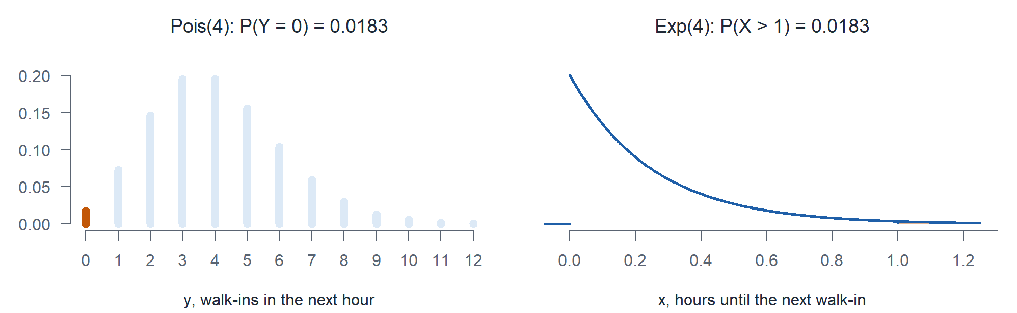
dpois(0, 4) = 0.0183
1 - pexp(1, 4) = 0.0183

---

What We’re Doing: Lesson 14

Objectives

• Summarize project data with appropriate graphical and numerical descriptive methods (histograms, boxplots, scatterplots). (SLO 2)
• Compute and interpret the sample correlation coefficient \(r\). (SLO 2)
• Distinguish correlation from causation. (SLO 6)
• Communicate exploratory findings and pose questions for further analysis. (SLO 1)

Required Reading

Supplement S3 (Canvas)

---

Break!

Family

1

2

3

---

The EDA

ImportantProject Event 1 of 4: EDA, 25 points, due 11 October

Your EDA is a report you publish in Vantage. We walk through it in class today.

• Plot and summarize every variable you plan to use before you model anything
• \(r\) measures the strength and direction of a linear association
• Correlation is not causation

Open Vantage

Go to the MA206 folder in Vantage.

NoteEDA Template

---
title: "MA206 Exploratory Data Analysis: Brigade Readiness"
subtitle: "AY27-1 Graded Milestone"
author: "PUT YOUR NAME HERE"
date: "`r Sys.Date()`"
output: html_document
---

```{r setup, include=FALSE}
knitr::opts_chunk$set(echo = TRUE, warning = FALSE, message = FALSE)
library(tidyverse)
library(foundry)
```

# Introduction

<!-- Replace the blank below with three or four sentences: which brigade you were assigned, what this report examines, and why readiness matters to a commander. -->

**YOUR INTRODUCTION:**

>

# The Data

```{r load}
master <- datasets.read_table("ay27_1_master")
```

## Unit Selected

<!-- Change the text below to the brigade you were assigned. The full list is in MA206_Available_Brigades.csv. -->

```{r filter}
MY_BRIGADE <- "173D AIRBORNE BRIGADE COMBAT TEAM"
bde <- master %>% filter(BrigadeName == MY_BRIGADE)
```

## Structure and Scope

<!-- Run the chunk below and read the output. Everything you need for the blanks is in it.-->

```{r inventory}
dim(master)
glimpse(bde)
summary(select(bde, age, time_in_active_service_years, height, weight, body_fat_percent, aft_score_total))
count(bde, battalion)
count(bde, company)
count(bde, sex)
count(bde, aft_pass)
```

## Key Figures

<!-- Read the output above and replace each blank with the number you find. -->

- Rows in the full dataset: **____**
- Columns in the full dataset: **____**
- Soldiers in my brigade: **____**
- Battalions in my brigade: **____**
- Companies in my brigade: **____**
- Mean age in my brigade: **____**
- Median AFT total score: **____**
- Number of women in my brigade: **____**
- Number who passed the AFT: **____**

<!-- One sentence: what surprised you in the output above? -->

>

# Readiness Findings

<!-- Each plot below is written for you. Run it, study it, and write two to three sentences underneath. Do not change the code. -->

## AFT Total Score Distribution

```{r plot1}
ggplot(bde, aes(x = aft_score_total)) + geom_histogram(bins = 30) +
  labs(title = paste("AFT total score:", MY_BRIGADE), x = "AFT total score", y = "Soldiers")
```

**Interpretation**

>

## AFT Score by Battalion

```{r plot2}
ggplot(bde, aes(x = battalion, y = aft_score_total)) + geom_boxplot() +
  coord_flip() + labs(title = "AFT total score by battalion", x = "Battalion", y = "AFT total score")
```

**Interpretation**

>

## AFT Pass Rate by Company

```{r plot3}
bde %>% group_by(company) %>%
  summarise(pass_rate = 100*mean(aft_pass, na.rm=TRUE), n = n()) %>%
  filter(n >= 10) %>%
  ggplot(aes(x = reorder(company, pass_rate), y = pass_rate)) + geom_col() +
  coord_flip() + labs(title = "AFT pass rate by company", x = "Company", y = "Percent passing")
```

**Interpretation**

>

## Time in Service and AFT Score

```{r plot4}
ggplot(bde, aes(x = time_in_active_service_years, y = aft_score_total)) +
  geom_point(alpha = 0.2) + geom_smooth(method = "lm") +
  labs(title = "Time in service versus AFT score", x = "Years of active service", y = "AFT total score")
```

**Interpretation**

>

# Further Analysis

<!-- Build three plots that the provided four did not cover. At least one must use a variable not used above. Useful columns: age, age_bracket, sex, height, weight, body_fat_percent, body_comp_pass, skill_level, aft_score_plank, aft_score_push_up, aft_score_2mi_run, aft_raw_deadlift, m4, pistol, m249. -->

<!-- For each: say why you chose it before the code, and what it shows after. -->

## Additional Analysis 1

**Question**

>

```{r myplot1}
# YOUR CODE HERE
```

**Finding**

>

## Additional Analysis 2

**Question**

>

```{r myplot2}
# YOUR CODE HERE
```

**Finding**

>

## Additional Analysis 3

**Question**

>

```{r myplot3}
# YOUR CODE HERE
```

**Finding**

>

# Summary and Recommendation

<!-- In one paragraph, tell a commander what you found. Name the single biggest readiness concern in your brigade, cite the specific number that supports it, and give one recommendation. -->



>

---

# Proposed Investigation

<!-- Given what you found above, name one question you would want to investigate with this data. State the question, why it matters, and which variables you would use. -->

**Research question**

>

**Why it matters**

>

**Variables I would use**

>

<!-- When you are finished: click Render, then publish or rebuild your report. -->

NoteAvailable Brigades

"BrigadeName"
"101ST AIRBORNE DIVISION ARTILLERY"
"101ST AIRBORNE DIVISION SUSTAINMENT COMMAND"
"108TH AIR DEFENSE ARTILLERY BRIGADE"
"10TH MOUNTAIN DIVISION ARTILLERY"
"10TH MOUNTAIN DIVISION SUSTAINMENT BRIGADE"
"116TH MILITARY INTELLIGENCE BRIGADE"
"11TH AIR DEFENSE ARTILLERY BRIGADE"
"11TH ARMORED CAVALRY REGIMENT"
"12TH COMBAT AVIATION BRIGADE"
"165TH INFANTRY BRIGADE"
"16TH COMBAT AVIATION BRIGADE"
"16TH SUSTAINMENT BDE"
"173D AIRBORNE BRIGADE COMBAT TEAM"
"17TH FIELD ARTILLERY BRIGADE"
"18TH FIELD ARTILLERY BRIGADE"
"18TH MILITARY POLICE BRIGADE"
"193D INFANTRY BRIGADE"
"1ST ARMORED DIVISION ARTILLERY"
"1ST ARMORED DIVISION SUSTAINMENT BRIGADE"
"1ST BRIGADE COMBAT TEAM, 101ST AIRBORNE DIVISION"
"1ST BRIGADE COMBAT TEAM, 10TH MOUNTAIN DIVISION"
"1ST BRIGADE COMBAT TEAM, 11TH AIRBORNE DIVISION"
"1ST BRIGADE COMBAT TEAM, 1ST ARMORED DIVISION"
"1ST BRIGADE COMBAT TEAM, 1ST CAVALRY DIVISION"
"1ST BRIGADE COMBAT TEAM, 1ST INFANTRY DIVISION"
"1ST BRIGADE COMBAT TEAM, 2D INFANTRY DIVISON"
"1ST BRIGADE COMBAT TEAM, 3D INFANTRY DIVISION"
"1ST BRIGADE COMBAT TEAM, 4TH INFANTRY DIVISION"
"1ST BRIGADE COMBAT TEAM, 82D AIRBORNE DIVISION"
"1ST CAVALRY DIVISION DIVARTY"
"1ST CAVALRY DIVISION SUSTAINMENT BRIGADE"
"1ST INFANTRY DIVISION ARTILLERY"
"1ST INFANTRY DIVISION SUSTAINMENT BRIGADE"
"1ST MEDICAL BRIGADE"
"20TH ENGINEER BRIGADE"
"210TH FIRES BDE"
"2D BRIGADE COMBAT TEAM 1ST CAVALRY DIVISION"
"2D BRIGADE COMBAT TEAM 2D INFANTRY DIVISION"
"2D BRIGADE COMBAT TEAM 3D INFANTRY DIVISION"
"2D BRIGADE COMBAT TEAM 82D AIRBORNE DIVISION"
"2D BRIGADE COMBAT TEAM, 101ST AIRBORNE DIVISION"
"2D BRIGADE COMBAT TEAM, 10TH MOUNTAIN DIVISION"
"2D BRIGADE COMBAT TEAM, 11TH AIRBORNE DIVISION"
"2D BRIGADE COMBAT TEAM, 1ST ARMORED DIVISION"
"2D BRIGADE COMBAT TEAM, 1ST INFANTRY DIVISION"
"2D BRIGADE COMBAT TEAM, 4TH INFANTRY DIVISION"
"2D CAVALRY REGIMENT (STRYKER)"
"2D INFANTRY DIVISION SUSTAINMENT BRIGADE"
"2LBCT [P], 25TH INFANTRY DIVISION"
"2ND AV BDE CAB HVY 2ID"
"31ST AIR DEFENSE ARTILLERY BRIGADE"
"35TH AIR DEFENSE ARTILLERY BDE"
"35TH SIGNAL BRIGADE"
"36TH ENGINEER BRIGADE"
"3D BRIGADE COMBAT TEAM 1ST CAVALRY DIVISION"
"3D BRIGADE COMBAT TEAM 82D AIRBORNE DIVISION"
"3D BRIGADE COMBAT TEAM, 101ST AIRBORNE DIVISION"
"3D BRIGADE COMBAT TEAM, 10TH MOUNTAIN DIVISION"
"3D BRIGADE COMBAT TEAM, 1ST ARMORED DIVISION"
"3D BRIGADE COMBAT TEAM, 4TH INFANTRY DIVISION"
"3D CAVALRY REGIMENT"
"3D INFANTRY DIVISION SUSTAINMENT BRIGADE"
"3IBCT, 25TH INFANTRY DIVISION"
"3ID DIVISION ARTILLERY"
"41ST FIELD ARTILLERY BRIGADE"
"44TH MEDICAL BRIGADE"
"48TH CHEMICAL BRIGADE"
"4TH INFANTRY DIVISION ARTILLERY"
"4TH INFANTRY DIVISION SUSTAINMENT BRIGADE"
"52D AIR DEFENSE ARTILLERY BRIGADE"
"62D MEDICAL BRIGADE"
"65TH MEDICAL BRIGADE"
"69TH AIR DEFENSE ARTILLERY BRIGADE"
"704TH MILITARY INTELLIGENCE BRIGADE"
"75TH FIELD ARTILLERY BRIGADE"
"780TH MILITARY INTELLIGENCE BRIGADE"
"7TH TRANSPORTATION BRIGADE (EXPEDITIONARY)"
"82D AIRBORNE DIVISION ARTILLERY"
"82D AIRBORNE DIVISION SUSTAINMENT COMMAND"
"89TH MILITARY POLICE BRIGADE"
"COMBAT AVIATION BRIGADE 101ST AIRBORNE DIVISION"
"COMBAT AVIATION BRIGADE 1ST ARMORED DIVISION"
"COMBAT AVIATION BRIGADE 1ST INFANTRY DIVISION"
"COMBAT AVIATION BRIGADE 3D INFANTRY DIVISION"
"COMBAT AVIATION BRIGADE 4TH INFANTRY DIVISION."
"COMBAT AVIATION BRIGADE 82D AIRBORNE DIVISION"
"COMBAT AVIATION BRIGADE, 10TH MOUNTAIN DIVISION"
"COMBAT AVIATION BRIGADE, 1ST CAVALRY DIVISION"
"COMBAT AVIATION BRIGADE, 25TH INFANTRY DIVISION"
"DIVISION ARTILLERY, 25TH INFANTRY DIVISION"
"HHB, 2D INFANTRY DIVISION ARTILLERY HQS"
"HQ, 434TH FIELD ARTILLERY BRIGADE"
"SUSTAINMENT BDE, 25TH INFANTRY DIVISION"
"U.S. ARMY ARCTIC AVIATION CMD"
"US ARMY 1ST RECRUITING BRIGADE"
"US ARMY 2D RECRUITING BRIGADE"
"US ARMY 3D RECRUITING BRIGADE"
"US ARMY 5TH RECRUITING BRIGADE"
"US ARMY 6TH RECRUITING BRIGADE"

Where We Are in the Project

Event	Lesson	Date	Points
EDA	14	Due 11 Oct	25
IPR	34	20-23 Nov	25
Products	37	3-4 Dec	50
Brief	38-39	7-10 Dec	100

---

Before You Leave

Today

• Count or wait: same rate, Poisson counts the events, exponential measures the waits

Any questions?

---

Next Lesson

Lesson 15: Cadet-Led Review

• Review Lessons 1-13

---

Upcoming Graded Events

• EDA: due 11 October
• WPR I: Lesson 16 (covers Lessons 1-13)
• TEE: 15-18 Dec 2026