Lesson 15: Cadet-Led Review
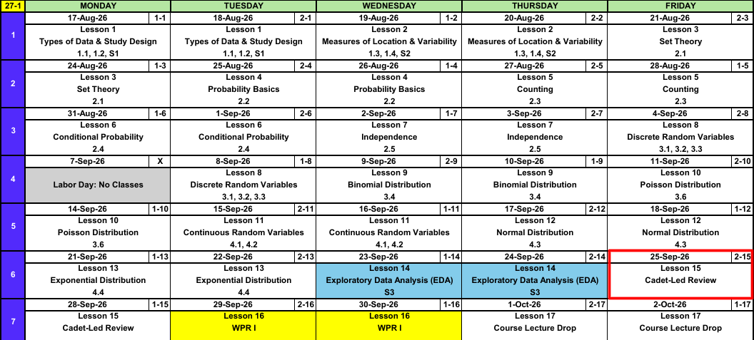
Calendar
WPR I Admin
ImportantWPR I: Lesson 16 (29, 30 Sep)
- Covers: Lessons 1 through 13
- Time: 55 minutes
- Authorized: the course statistics reference card (SRC), R-Lite, and the issued calculator
R-Lite and the SRC
Study Materials
- WPR I Review and Solutions
- Last semester, for more practice: WPR I Review (AY26-2) and Solutions
What We’re Doing: Lesson 15
Objectives
- Review Lessons 1-13.
Required Reading
None
Break!
Family

Cadet-Led Review
Block I Outline
Descriptive Statistics
Lesson 1: Types of Data & Study Design (Devore 1.1, 1.2, S1)
- Population, sample, and process
- Descriptive vs inferential statistics
- Parameter (\(\mu\), \(\sigma\), \(p\)) vs statistic (\(\bar{x}\), \(s\), \(\hat{p}\))
- Categorical (nominal, ordinal) vs numerical (discrete, continuous)
- Histograms and shape: symmetric, skewed left, skewed right (named for the tail)
- Simple random sample
- Observational study vs experiment
- Random sampling buys generalization, random assignment buys causation
Lesson 2: Measures of Location & Variability (Devore 1.3, 1.4, S2)
- Center: mean \(\bar{x}\), median \(\tilde{x}\), trimmed mean
- Mean is sensitive to outliers, median is resistant
- Spread: range, sample variance \(s^2 = \dfrac{\sum (x_i - \bar{x})^2}{n - 1}\), standard deviation \(s\)
- Fourth spread \(f_s\) = upper fourth minus lower fourth
- Outlier: more than \(1.5 f_s\) beyond the nearest fourth, extreme beyond \(3 f_s\)
- Boxplots and comparative boxplots
Probability
Lesson 3: Set Theory (Devore 2.1)
- Experiment, sample space \(\mathcal{S}\), event (a subset of \(\mathcal{S}\))
- Union \(A \cup B\) (“or”), intersection \(A \cap B\) (“and”), complement \(A'\) (“not”)
- Mutually exclusive (disjoint): \(A \cap B = \emptyset\)
- Venn diagrams
- DeMorgan’s laws: \((A \cup B)' = A' \cap B'\) and \((A \cap B)' = A' \cup B'\)
Lesson 4: Probability Basics (Devore 2.2)
- Axioms: \(P(A) \ge 0\), \(P(\mathcal{S}) = 1\), and disjoint probabilities add
- Complement rule: \(P(A') = 1 - P(A)\)
- Addition rule: \(P(A \cup B) = P(A) + P(B) - P(A \cap B)\), and its three event version
- Equally likely outcomes: \(P(A) = N(A)/N\)
- Two way tables
Lesson 5: Counting (Devore 2.3)
- Product rule: \(n_1 n_2 \cdots n_k\)
- Permutation (order matters): \(P_{k,n} = \dfrac{n!}{(n-k)!}\)
- Combination (order does not): \(\dbinom{n}{k} = \dfrac{n!}{k!\,(n-k)!}\)
- Counting to get probabilities: \(P(A) = N(A)/N\)
Lesson 6: Conditional Probability (Devore 2.4)
- Conditional probability: \(P(A \mid B) = \dfrac{P(A \cap B)}{P(B)}\)
- Multiplication rule: \(P(A \cap B) = P(A \mid B)\,P(B)\)
- Tree diagrams
- Law of Total Probability: \(P(B) = \sum_i P(B \mid A_i)\,P(A_i)\)
- Bayes’ Theorem: \(P(A_j \mid B) = \dfrac{P(B \mid A_j)\,P(A_j)}{\sum_i P(B \mid A_i)\,P(A_i)}\)
Lesson 7: Independence (Devore 2.5)
- Independent: \(P(A \mid B) = P(A)\)
- Test with \(P(A \cap B) = P(A)\,P(B)\)
- Independent is not the same as mutually exclusive
- \(P(\text{at least one}) = 1 - P(\text{none})\)
- Counting combined with independence
Random Variables
Lesson 8: Discrete Random Variables (Devore 3.1, 3.2, 3.3)
- Random variable: a number assigned to each outcome
- pmf: \(p(x) = P(X = x)\), with \(p(x) \ge 0\) and \(\sum_x p(x) = 1\)
- cdf: \(F(x) = P(X \le x)\), a step function
- Expected value: \(E(X) = \mu = \sum_x x\,p(x)\)
- Variance: \(V(X) = \sigma^2 = E(X^2) - [E(X)]^2\), and \(\sigma = \sqrt{V(X)}\)
Lesson 9: Binomial Distribution (Devore 3.4)
- BINS: binary outcomes, independent trials, fixed \(n\), same \(p\)
- \(X \sim \text{Bin}(n, p)\) counts successes
- pmf: \(p(x) = \dbinom{n}{x} p^x (1-p)^{n-x}\) for \(x = 0, 1, \ldots, n\)
- \(E(X) = np\) and \(V(X) = np(1-p)\)
- R-Lite:
dbinomis the pmf,pbinomis the cdf - Fully specify: name the variable, name the distribution, give the parameters
Lesson 10: Poisson Distribution (Devore 3.6)
- Counts events over a window: time, distance, or area
- Poisson process: rate \(\lambda\), window \(t\), so \(\mu = \lambda t\)
- pmf: \(p(x; \mu) = \dfrac{e^{-\mu}\mu^x}{x!}\) for \(x = 0, 1, 2, \ldots\)
- \(E(X) = V(X) = \mu\)
- R-Lite:
dpoisis the pmf,ppoisis the cdf
Lesson 11: Continuous Random Variables (Devore 4.1, 4.2)
- pdf: \(f(x) \ge 0\) and \(\int_{-\infty}^{\infty} f(x)\,dx = 1\)
- Probability is area: \(P(a \le X \le b) = \int_a^b f(x)\,dx\)
- \(P(X = c) = 0\), so \(\le\) and \(<\) give the same answer
- cdf: \(F(x) = P(X \le x) = \int_{-\infty}^{x} f(y)\,dy\), and \(P(a \le X \le b) = F(b) - F(a)\)
- Percentile: solve \(F(c) = P(X \le c) = p\) for \(c\)
- \(E(X) = \int x\,f(x)\,dx\) and \(V(X) = E(X^2) - [E(X)]^2\)
Lesson 12: Normal Distribution (Devore 4.3)
- \(X \sim N(\mu, \sigma^2)\): symmetric, bell shaped, centered at \(\mu\)
- Standard normal: \(Z \sim N(0, 1)\)
- Standardize: \(z = \dfrac{x - \mu}{\sigma}\), then use the \(z\) table
- Percentiles: \(x = \mu + z\sigma\)
- Critical value: \(z_\alpha\) has area \(\alpha\) to its right
- Empirical rule: 68%, 95%, 99.7% within 1, 2, 3 standard deviations
- R-Lite:
pnorm(x, mean, sd)is the cdf,qnormruns it backwards
Lesson 13: Exponential Distribution (Devore 4.4)
- \(X \sim \text{Exp}(\lambda)\) models a wait
- pdf: \(f(x) = \lambda e^{-\lambda x}\) for \(x \ge 0\)
- cdf: \(F(x) = P(X \le x) = 1 - e^{-\lambda x}\), so \(P(X > x) = e^{-\lambda x}\)
- \(E(X) = \sigma = 1/\lambda\)
- Memoryless: \(P(X \ge t + t_0 \mid X \ge t_0) = P(X \ge t)\)
- Poisson counts events at rate \(\lambda\), the waits between them are \(\text{Exp}(\lambda)\)
- R-Lite:
pexp(x, rate)takes the rate, not the mean
Distributions
| Binomial | Poisson | Normal | Exponential | |
|---|---|---|---|---|
| Type | Discrete | Discrete | Continuous | Continuous |
| Use it when | \(x\) successes in \(n\) fixed trials | \(x\) events in a window | Symmetric, bell shaped measurement | Wait until the next event |
| Fully specified | \(X \sim \text{Binom}(n,\ p)\) | \(X \sim \text{Pois}(\mu)\) | \(X \sim N(\mu,\ \sigma^2)\) | \(X \sim \text{Exp}(\lambda)\) |
| Parameters | \(n\) trials, \(p\) success probability | \(\mu = \lambda t\), expected count | \(\mu\) center, \(\sigma\) spread | \(\lambda\) rate |
| Possible values | \(x = 0, 1, \dots, n\) | \(x = 0, 1, 2, \dots\) | \(-\infty < x < \infty\) | \(x \ge 0\) |
| pmf or pdf | \(\dbinom{n}{x} p^x (1-p)^{n-x}\) | \(\dfrac{e^{-\mu}\mu^x}{x!}\) | \(\dfrac{1}{\sqrt{2\pi}\,\sigma} e^{-(x-\mu)^2/(2\sigma^2)}\) | \(\lambda e^{-\lambda x}\) |
| \(E(X)\) | \(np\) | \(\mu\) | \(\mu\) | \(1/\lambda\) |
| \(V(X)\) | \(np(1-p)\) | \(\mu\) | \(\sigma^2\) | \(1/\lambda^2\) |
d, the pmf or pdf |
dbinom(x, n, p) |
dpois(x, mu) |
dnorm(x, mean, sd) |
dexp(x, rate) |
p, the cdf \(P(X \le x)\) |
pbinom(x, n, p) |
ppois(x, mu) |
pnorm(x, mean, sd) |
pexp(x, rate) |
q, the cdf backwards |
qbinom(area, n, p) |
qpois(area, mu) |
qnorm(area, mean, sd) |
qexp(area, rate) |
Problem 1: Saturday Run
The distance \(X\) (in miles) a cadet runs on a Saturday morning has pdf
\[f(x) = \begin{cases} \dfrac{x}{24} & 1 \le x \le 7 \\ 0 & \text{otherwise} \end{cases}\]
NoteQuestions
- Find the cdf \(F(x) = P(X \le x)\) and write it in full piecewise form.
- Find \(P(X < 3)\).
- Find \(P(X \le 3)\).
- Find \(P(X > 6)\).
- Find \(P(X \ge 6)\).
- Find \(P(X = 6)\).
- Find \(\mu\) and \(\sigma\). Then find the probability \(X\) is within one standard deviation of its mean.
TipAnswers
- For \(1 \le x \le 7\), \(\displaystyle\int_1^x \frac{y}{24}\,dy = \frac{x^2 - 1}{48}\), so
\[F(x) = P(X \le x) = \begin{cases} 0 & x < 1 \\ \dfrac{x^2 - 1}{48} & 1 \le x \le 7 \\ 1 & x > 7 \end{cases}\]
\(F(3) = \dfrac{9 - 1}{48} = \dfrac{1}{6} \approx \mathbf{0.167}\)
\(F(3) \approx \mathbf{0.167}\), the same as (b), because \(P(X = 3) = 0\).
\(1 - F(6) = 1 - \dfrac{36 - 1}{48} = \dfrac{13}{48} \approx \mathbf{0.271}\)
\(1 - F(6) \approx \mathbf{0.271}\), the same as (d).
\(\mathbf{0}\). A single value has no area under the pdf. That is why (d) and (e) are equal.
\(\mu = \displaystyle\int_1^7 x \cdot \frac{x}{24}\,dx = \frac{343 - 1}{72} = 4.75\) and \(E(X^2) = \displaystyle\int_1^7 x^2 \cdot \frac{x}{24}\,dx = \frac{2401 - 1}{96} = 25\), so \(V(X) = 25 - 4.75^2 = 2.4375\) and \(\sigma \approx 1.561\).
\(\mu \pm \sigma \approx (3.189,\ 6.311)\), so \(P(3.189 < X < 6.311) = F(6.311) - F(3.189) = \dfrac{6.311^2 - 3.189^2}{48} \approx \mathbf{0.618}\)
Problem 2: Motor Pool Work Orders
Work orders arrive at a battalion motor pool randomly and independently at an average rate of 5 per hour. Let \(X\) be the number of work orders in 1 hour.
NoteQuestions
- Fully specify the distribution of \(X\).
- Find \(P(X < 3)\).
- Find \(P(X \le 3)\).
- Find \(P(X > 7)\).
- Find \(P(X \ge 7)\).
- Find \(\mu\) and \(\sigma\). Then find the probability \(X\) is within one standard deviation of its mean.
TipAnswers
\(X \sim \text{Pois}(\mu = 5)\) work orders per hour.
\(P(X < 3) = P(X \le 2) = F(2) \approx \mathbf{0.125}\)
ppois(2, 5)\(F(3) \approx \mathbf{0.265}\)
ppois(3, 5)\(1 - P(X \le 7) = 1 - F(7) \approx \mathbf{0.133}\)
1 - ppois(7, 5)\(1 - P(X \le 6) = 1 - F(6) \approx \mathbf{0.238}\)
1 - ppois(6, 5)\(\mu = 5\) and \(\sigma = \sqrt{5} \approx 2.236\). \(\mu \pm \sigma \approx (2.764,\ 7.236)\), so \(P(3 \le X \le 7) = F(7) - F(2) \approx \mathbf{0.742}\)
ppois(7, 5) - ppois(2, 5)
Problem 3: Motor Pool Work Orders, Continued
Same motor pool, work orders still arrive at 5 per hour. Now let \(T\) be the time (in hours) between one work order and the next.
NoteQuestions
- Fully specify the distribution of \(T\). Write its pdf. Then find the cdf \(F(t) = P(T \le t)\) and write it in full piecewise form.
- Find \(P(T < 0.2)\).
- Find \(P(T \le 0.2)\).
- Find \(P(T > 0.5)\).
- Find \(P(T \ge 0.5)\).
- Find \(P(T = 0.5)\).
- Find \(\mu\) and \(\sigma\). Then find the probability \(T\) is more than two standard deviations above its mean.
- Find the 90th percentile of \(T\).
TipAnswers
- The wait between Poisson events is exponential, so \(T \sim \text{Exp}(\lambda = 5)\) with \(f(t) = 5e^{-5t}\) for \(t \ge 0\). For \(t \ge 0\), \(\displaystyle\int_0^t 5e^{-5s}\,ds = 1 - e^{-5t}\), so
\[F(t) = P(T \le t) = \begin{cases} 0 & t < 0 \\ 1 - e^{-5t} & t \ge 0 \end{cases}\]
\(F(0.2) = 1 - e^{-1} \approx \mathbf{0.632}\)
pexp(0.2, 5)\(F(0.2) \approx \mathbf{0.632}\), the same as (b).
\(1 - F(0.5) = e^{-2.5} \approx \mathbf{0.082}\)
1 - pexp(0.5, 5)\(1 - F(0.5) \approx \mathbf{0.082}\), the same as (d).
\(\mathbf{0}\). A single value has no area under the pdf. That is why (d) and (e) are equal.
\(\mu = \sigma = 1/\lambda = 0.2\) hours. \(\mu + 2\sigma = 0.6\), so \(P(T > 0.6) = 1 - F(0.6) = e^{-3} \approx \mathbf{0.050}\)
1 - pexp(0.6, 5)Solve \(F(c) = P(T \le c) = 0.90\) for \(c\):
\[1 - e^{-5c} = 0.90 \quad\Rightarrow\quad e^{-5c} = 0.10 \quad\Rightarrow\quad c = \frac{\ln(10)}{5} \approx \mathbf{0.461} \text{ hours}\]
qexp(0.90, 5)
Before You Leave
Today
- Review Lessons 1-13
Any questions?
Next Lesson
- Covers Lessons 1-13
Upcoming Graded Events
- WPR I: Lesson 16 (covers Lessons 1-13)
- EDA: due 11 October
- TEE: 15-18 Dec 2026