

Lesson 29: PCA, How Many to Keep

Calendar

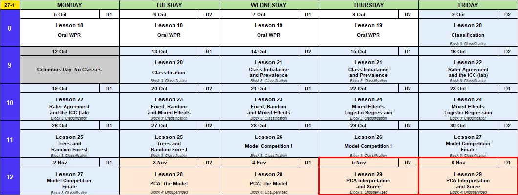
Calendar for 5 October to 6 November with red boxes around Thursday 5 November and Friday 6 November, Lesson 29, PCA Interpretation and Scree.

Admin

This Lesson

  • Data: USArrests ships with R. Practice data: L29_cadet_fitness.csv.
  • Reading: ISLR pages 503 to 505 and 507 to 508.

Coming Up

  • Lesson 30, k-means clustering. A1, BC1 Mon 9 Nov; BC2 Tue 10 Nov. MAJ Semmel is back.
  • Capstone Milestone 2: methodology and preliminary results. Due 2359 Friday 13 November, 60 points.
  • Capstone final presentation. Lessons 37 and 38, 3 to 8 December, 100 points.

TEE Slots

All TEE periods run 0730 to 1100. Find your name under your section.

P1: Tue 15 Dec (8) P4: Wed 16 Dec (7)
Anteen Baron
Carroll Fountain
Cole Hardwick
Fonte Rebolledo
Konopka Shioutakon
Ploetz Smith
Sun Youmans
Toth  
P1: Tue 15 Dec (5) P4: Wed 16 Dec (9)
Bode Best
Lee De La Torre
Ndiaye Laub
O’Keefe Loughman
Russell Miranda
  Nguyen
  Plummer
  Ward
  Weisenborn
P1: Tue 15 Dec (4) P4: Wed 16 Dec (11)
Gray Applegate
Harris Cannon
Van Kley Ivey
Zhai Johnson
  Kendig
  Marino
  Myers
  Silverman
  Song
  Tullier
  Wittrock

Break!

Army

Subdued Sapper tab. Ranger tab.


What We Did: Lessons 20 to 28

Truth positive Truth negative
Predicted positive TP FP, a false alarm
Predicted negative FN, a miss TN
  • Accuracy \(= \dfrac{TP + TN}{n}\)
  • Sensitivity (recall) \(= \dfrac{TP}{TP + FN}\), specificity \(= \dfrac{TN}{TN + FP}\)
  • Precision \(= \dfrac{TP}{TP + FP}\)
  • \(F_1 = \dfrac{2\,TP}{2\,TP + FP + FN}\)
  • Cut probabilities into labels at a threshold. \(0.5\) is a default, not a rule.
  • Rare outcome: the null classifier scores \(1 - \text{prevalence}\), and a \(0.5\) threshold flags almost nothing.
  • Three fixes: move the threshold, class weights (glm(..., weights = w)), undersample. Each one moves the cutoff. None improves the model.
  • Sensitivity and specificity do not move with prevalence. Precision does.
  • Report performance with the prevalence it was measured at.
  • Percent agreement \(p_o\). Chance agreement \(p_e = P(A)P(B) + P(A^c)P(B^c)\)
  • Cohen’s kappa \(\kappa = \dfrac{p_o - p_e}{1 - p_e}\): agreement once you remove chance. Falls as prevalence moves to an extreme.
  • \(\text{PABAK} = 2p_o - 1\): kappa with the prevalence set at half
  • ICC \(= \dfrac{\hat\sigma^2_{\text{subject}}}{\hat\sigma^2_{\text{subject}} + \hat\sigma^2_{\text{rater}} + \hat\sigma^2_{\text{error}}}\), from a two-way ANOVA with raters as blocks
  • Reliability is not validity: raters can agree and all be wrong.
  • \(y_{ij} = \mu + u_j + \varepsilon_{ij}\), \(u_j \sim N(0, \sigma^2_u)\), \(\varepsilon_{ij} \sim N(0, \sigma^2)\)
  • lmer(y ~ 1 + (1 | group), data = d), then fixef(), ranef(), coef()
  • \(\hat y_{ij} = \hat\mu + w_j(\bar y_j - \hat\mu)\), \(w_j = \dfrac{n_j}{n_j + \lambda}\), \(\lambda = \dfrac{\hat\sigma^2}{\hat\sigma^2_u}\): small groups shrink toward the average
  • \(\text{ICC} = \dfrac{\hat\sigma^2_u}{\hat\sigma^2_u + \hat\sigma^2}\)
  • Fixed: these levels are all you care about. Random: the levels are a sample of many.
  • \(\log\dfrac{p_{ij}}{1 - p_{ij}} = \mu + u_j\), \(u_j \sim N(0, \sigma^2_u)\). No \(\varepsilon\): pass or fail is the noise.
  • glmer(y ~ x + (1 | group), family = binomial, data = d)
  • predict(fit, newdata, type = "response", allow.new.levels = TRUE)
  • glm with a dummy per group: a group at 100% gets \(\hat\beta \to \infty\). glmer shrinks it.
  • \(\text{ICC} = \dfrac{\hat\sigma^2_u}{\hat\sigma^2_u + \pi^2/3}\)
  • A tree splits the data into boxes. Each split picks the predictor and cut that lowers Gini impurity the most.
  • Gini for a box: \(G = 2p(1 - p)\). After a split, average the two boxes, weighted by size.
  • A tree grown all the way memorizes the training data and does worse on new data. Limit it.
  • Random forest: many trees, each on a bootstrap sample, each split choosing from mtry random predictors. The forest votes.
  • randomForest(y ~ ., data = train, ntree = , mtry = , nodesize = ); tune on out-of-bag \(F_1\).
  • predict(fit, newdata, type = "prob") gives the share of trees that vote yes.
  • Variable importance says which predictors the forest leans on, not how.
  • Six model types on the Memo 4 leads, scored on \(F_1\) of the call column.
  • Logistic at \(0.5\) calls nobody: about 97% accurate, \(F_1 = 0\).
  • Tune the cut on train (five-fold cross-validation) or on the forest’s out-of-bag votes. Never on test.
  • Check on test, then refit on all 12,000 before you predict the incoming leads.
  • Calls \(= TP + FP\). The recruiters can make 1,230.
  • No \(y\). PCA builds new columns from the \(x\)’s: \(Z_m = \phi_{1m} X_1 + \phi_{2m} X_2 + \dots + \phi_{pm} X_p\)
  • Loadings \(\phi\): squares sum to 1. \(Z_1\) is as spread out as possible; \(Z_2\) the same, uncorrelated with \(Z_1\); and so on.
  • pca <- prcomp(d, scale. = TRUE): pca$rotation loadings, pca$x scores, summary(pca) shares
  • Scale first. Scaled, the total variance is the number of columns.
  • The sign of a component is arbitrary. Read each \(Z\) by its biggest loadings.
  • Biplot: dots are scores, arrows are loadings.

What We’re Doing: Lesson 29

Where We Left Off

The Lesson 28 fit:

arrests <- as_tibble(USArrests, rownames = "state")
crime <- arrests |> select(-state)

pca <- prcomp(crime, scale. = TRUE)

# flip Z1 so a higher score = more crime
pca$rotation[, 1] <- -pca$rotation[, 1]
pca$x[, 1] <- -pca$x[, 1]

summary(pca)
Importance of components:
                          PC1    PC2     PC3     PC4
Standard deviation     1.5749 0.9949 0.59713 0.41645
Proportion of Variance 0.6201 0.2474 0.08914 0.04336
Cumulative Proportion  0.6201 0.8675 0.95664 1.00000
  • Four columns in, four \(Z\)’s out. \(Z_1\) and \(Z_2\) keep 86.8%.
  • \(Z_3\) and \(Z_4\) are small leftovers. Do we need them?
  • Today: how many components to keep.

Proportion of Variance Explained

Scaled, each column has variance 1, so the total is \(p = 4\).

\[ \text{PVE}_m = \frac{\text{Var}(Z_m)}{\text{total}} = \frac{\text{Var}(Z_m)}{p} \]

  • In summary(pca) above, Proportion of Variance is the PVE. Cumulative Proportion is the running total.

How Many Do We Keep?

  • PCA gives as many \(Z\)’s as columns: 4 here. Keep all 4 and we still have 4 numbers per state. Nothing gained.
  • The point is fewer numbers: keep the top few \(Z\)’s, drop the rest.
  • Each one we drop loses its PVE. So keep enough to hold most of the variance, and stop when the next one adds little.
  • How do we see where to stop?

The Scree Plot

pve_tbl <- tibble(component  = 1:4,
                  pve        = summary(pca)$importance["Proportion of Variance", ],
                  cumulative = summary(pca)$importance["Cumulative Proportion", ])

pve_tbl |>
  pivot_longer(c(pve, cumulative), names_to = "type") |>
  mutate(type = if_else(type == "pve", "PVE", "Cumulative PVE")) |>
  ggplot(aes(component, value)) +
  geom_line() +
  geom_point(size = 3) +
  facet_wrap(~ fct_rev(type)) +
  scale_y_continuous(limits = c(0, 1), labels = scales::percent) +
  labs(x = "Principal component", y = NULL) +
  theme_minimal()

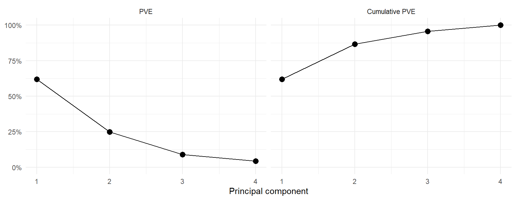
  • Left: the scree plot. Look for the elbow, where the drop flattens out.
  • Here it bends at 2: after \(Z_2\) each one adds little.
  • Right: two components keep 86.8%; three keep 95.7%.
  • No single right answer. ISLR: eyeball the elbow, and keep components you can interpret.

Scree is the pile of loose rock at the bottom of a cliff. The plot looks like a cliff, then the rubble.

What If We Hadn’t Scaled?

Same data, one change:

pca_raw <- prcomp(crime, scale. = FALSE)
summary(pca_raw)
Importance of components:
                           PC1      PC2    PC3     PC4
Standard deviation     83.7324 14.21240 6.4894 2.48279
Proportion of Variance  0.9655  0.02782 0.0058 0.00085
Cumulative Proportion   0.9655  0.99335 0.9991 1.00000
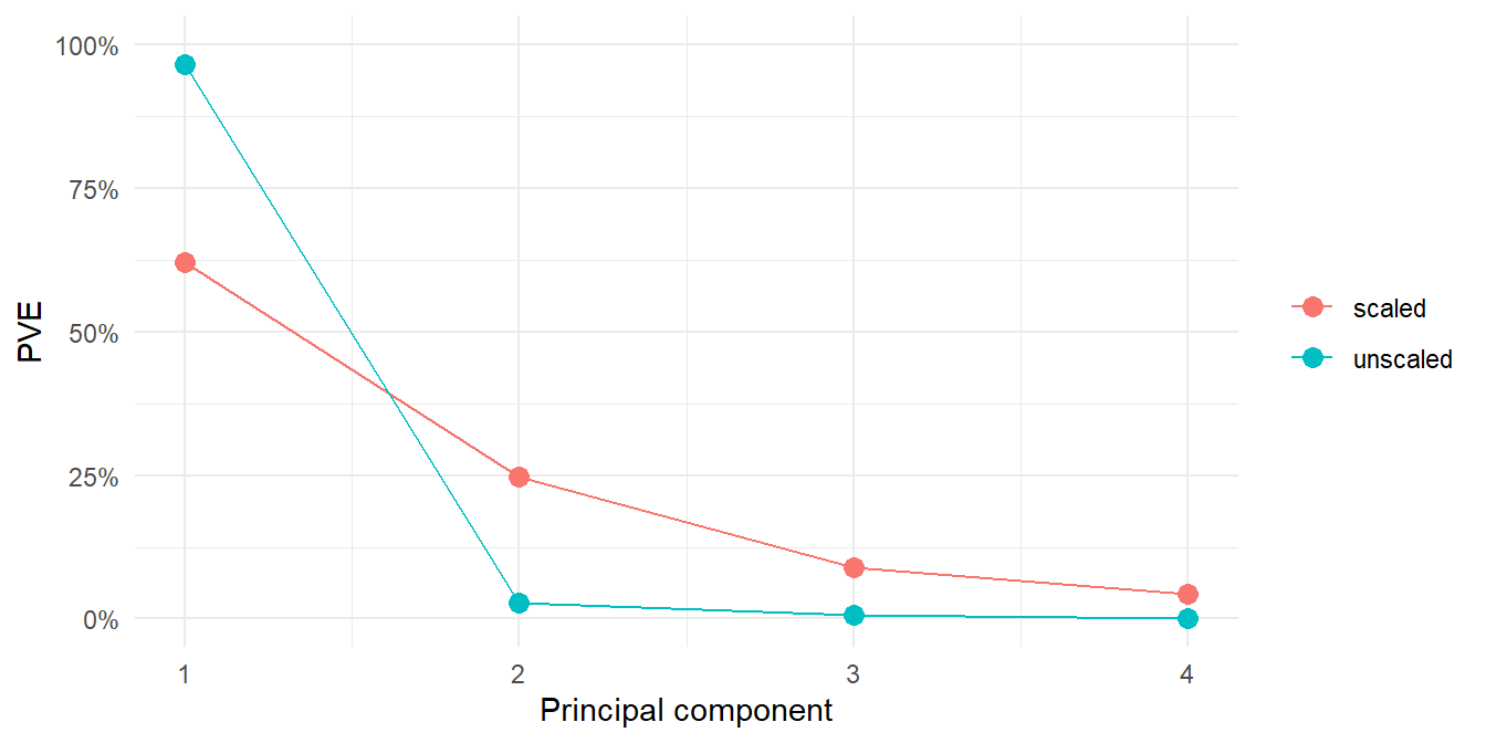
  • \(Z_1\) keeps 96.6%, not 62.0%. Better?

Side by Side: Share Kept

compare <- tibble(component = 1:4,
                  scaled   = summary(pca)$importance["Proportion of Variance", ],
                  unscaled = summary(pca_raw)$importance["Proportion of Variance", ])
compare
# A tibble: 4 × 3
  component scaled unscaled
      <int>  <dbl>    <dbl>
1         1 0.620   0.966  
2         2 0.247   0.0278 
3         3 0.0891  0.0058 
4         4 0.0434  0.00085
compare |>
  pivot_longer(c(scaled, unscaled), names_to = "fit", values_to = "pve") |>
  ggplot(aes(component, pve, color = fit)) +
  geom_line() +
  geom_point(size = 3) +
  scale_y_continuous(limits = c(0, 1), labels = scales::percent) +
  labs(x = "Principal component", y = "PVE", color = NULL) +
  theme_minimal()


Your Turn: Who Are the Fittest Cadets?

L29_cadet_fitness.csv: 240 cadets (simulated), 20 measures each, plus pps and set for later. Leave those two out of the PCA.

Group Columns Better is
AFT events (points) aft_deadlift, aft_pushups, aft_sdc, aft_plank, aft_run higher
Strength bench_lb, squat_lb, pullups, grip_kg higher
Endurance ruck_min (12-mile), swim_sec, resting_hr lower
vo2max higher
Speed and power dash40_sec, ioct_sec lower
vertical_in, broad_in higher
Body height_in, weight_lb neither
bodyfat_pct lower
fitness <- read_csv("data/L29_cadet_fitness.csv")

1. Look at the Correlations

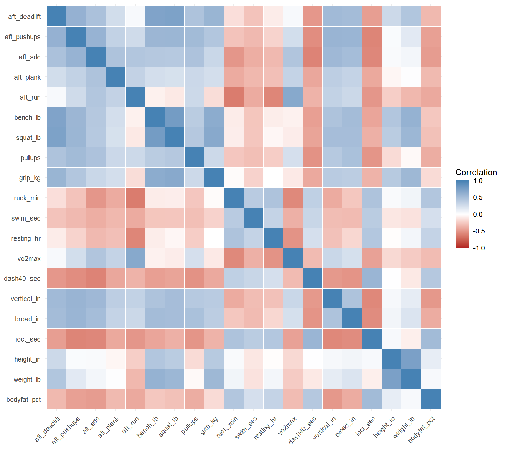
Plot the correlation matrix of the 20 columns. What do you see?

Code
measures <- fitness |> select(-cadet, -pps, -set)
cols <- names(measures)

cor(measures) |>
  as_tibble(rownames = "x") |>
  pivot_longer(-x, names_to = "y", values_to = "r") |>
  mutate(x = factor(x, levels = cols), y = factor(y, levels = rev(cols))) |>
  ggplot(aes(x, y, fill = r)) +
  geom_tile(color = "white") +
  scale_fill_gradient2(low = "firebrick", mid = "white", high = "steelblue", limits = c(-1, 1)) +
  labs(x = NULL, y = NULL, fill = "Correlation") +
  theme_minimal() +
  theme(axis.text.x = element_text(angle = 45, hjust = 1))

  • Almost every pair is correlated: fit cadets are good at most things.
  • Times, resting heart rate and body fat are red against the rest: lower is better.
  • Blocks: the lifts go together, the endurance columns go together, height and weight go together.
  • 20 columns, but a few things behind them. Which cadets are fittest overall? PCA builds that number.

2. Fit PCA

Fit PCA on the 20 columns, scaled. Then summary().

Code
pca_fit <- prcomp(fitness |> select(-cadet, -pps, -set), scale. = TRUE)
summary(pca_fit)
Importance of components:
                          PC1    PC2     PC3     PC4     PC5    PC6     PC7
Standard deviation     2.7579 1.9424 1.19979 0.87537 0.85544 0.7758 0.76987
Proportion of Variance 0.3803 0.1887 0.07197 0.03831 0.03659 0.0301 0.02963
Cumulative Proportion  0.3803 0.5689 0.64092 0.67923 0.71582 0.7459 0.77555
                           PC8    PC9    PC10    PC11    PC12    PC13    PC14
Standard deviation     0.72621 0.7127 0.68954 0.64423 0.61234 0.58968 0.58515
Proportion of Variance 0.02637 0.0254 0.02377 0.02075 0.01875 0.01739 0.01712
Cumulative Proportion  0.80192 0.8273 0.85109 0.87184 0.89059 0.90797 0.92509
                          PC15    PC16    PC17    PC18    PC19    PC20
Standard deviation     0.56303 0.54599 0.52192 0.47646 0.44185 0.43402
Proportion of Variance 0.01585 0.01491 0.01362 0.01135 0.00976 0.00942
Cumulative Proportion  0.94094 0.95585 0.96947 0.98082 0.99058 1.00000

3. How Many Do We Keep?

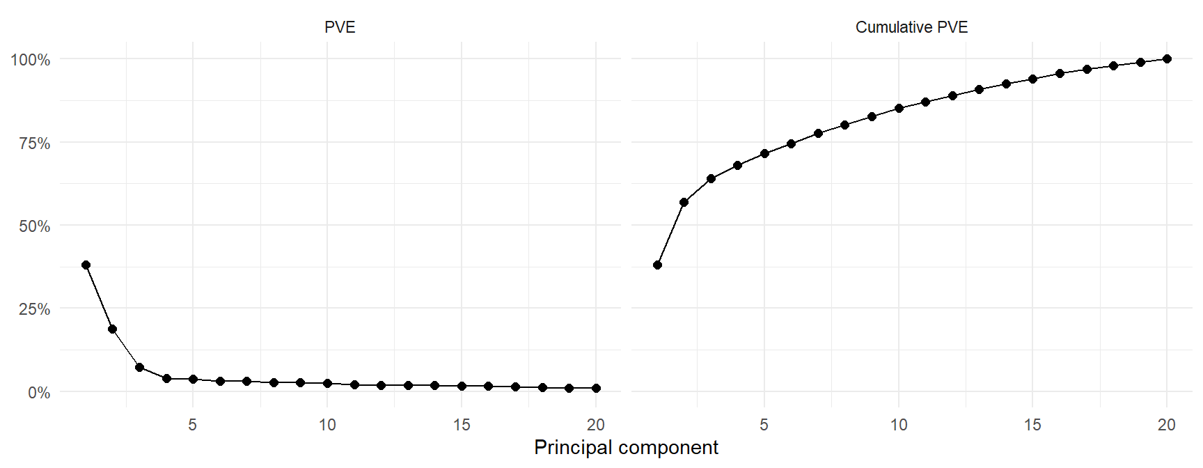
Draw the scree plot and the cumulative PVE. Where is the elbow?

Code
tibble(component  = 1:20,
       pve        = summary(pca_fit)$importance["Proportion of Variance", ],
       cumulative = summary(pca_fit)$importance["Cumulative Proportion", ]) |>
  pivot_longer(c(pve, cumulative), names_to = "type") |>
  mutate(type = if_else(type == "pve", "PVE", "Cumulative PVE")) |>
  ggplot(aes(component, value)) +
  geom_line() +
  geom_point(size = 2) +
  facet_wrap(~ fct_rev(type)) +
  scale_y_continuous(limits = c(0, 1), labels = scales::percent) +
  labs(x = "Principal component", y = NULL) +
  theme_minimal()

  • The elbow is at 3. \(Z_1\), \(Z_2\), \(Z_3\) keep 38.0%, 18.9%, 7.2%: 64.1% together.
  • After \(Z_3\), none keeps more than 3.8%. Keep 3, drop 17.

4. Is \(Z_1\) Fitness?

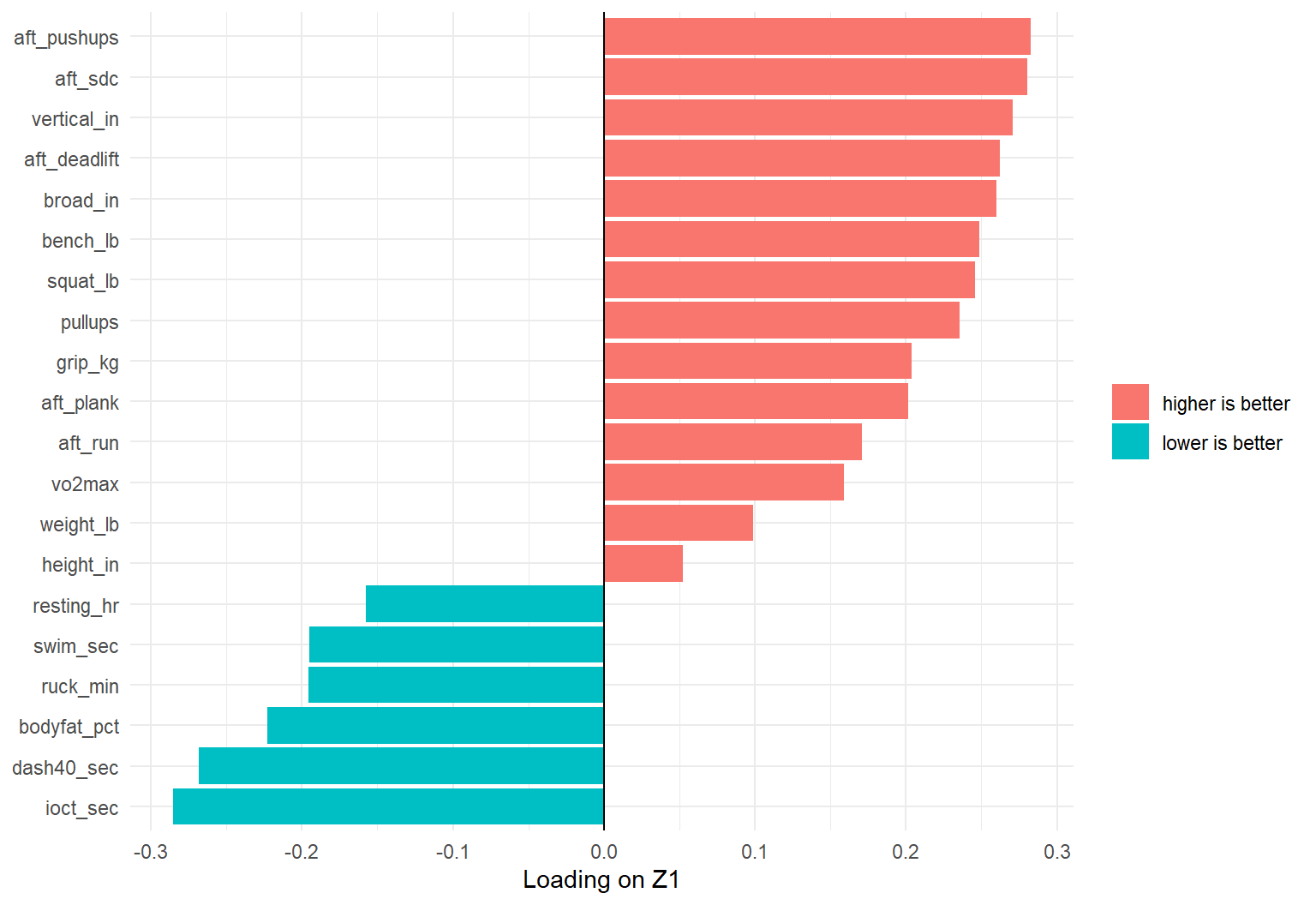
Plot the \(Z_1\) loadings. Do they point the “better” way for every column?

Code
lower_better <- c("ruck_min", "swim_sec", "resting_hr", "dash40_sec", "ioct_sec", "bodyfat_pct")

as_tibble(pca_fit$rotation[, 1:3], rownames = "column") |>
  mutate(better = if_else(column %in% lower_better, "lower is better", "higher is better"),
         column = fct_reorder(column, PC1)) |>
  ggplot(aes(PC1, column, fill = better)) +
  geom_col() +
  geom_vline(xintercept = 0) +
  labs(x = "Loading on Z1", y = NULL, fill = NULL) +
  theme_minimal()

  • Every higher-is-better column points one way. Every lower-is-better column points the other. \(Z_1\) is overall fitness.
  • Height and weight sit near 0: \(Z_1\) is not size.
  • If yours is backward (times positive), R flipped the sign. Multiply \(Z_1\) by \(-1\).
  • \(Z_2\): lifts and weight against the run and VO2 max, strength vs endurance. \(Z_3\): height and weight, body size.

5. Rank the Cadets

Who are the five fittest cadets on \(Z_1\)? Are they the best at any one thing?

Code
# flip if needed so a higher Z1 = fitter (IOCT time should load negative)
if (pca_fit$rotation["ioct_sec", 1] > 0) pca_fit$x[, 1] <- -pca_fit$x[, 1]

fitness |>
  bind_cols(as_tibble(pca_fit$x[, 1:3])) |>
  slice_max(PC1, n = 5) |>
  select(cadet, PC1, aft_run, squat_lb, ioct_sec, ruck_min)
# A tibble: 5 × 6
  cadet   PC1 aft_run squat_lb ioct_sec ruck_min
  <chr> <dbl>   <dbl>    <dbl>    <dbl>    <dbl>
1 C022   7.10      82      448      131      159
2 C163   6.65     100      342      101      149
3 C157   6.51      89      402      129      124
4 C193   6.44     100      402      127      158
5 C112   6.24      71      465      119      141
  • The top five are good at everything: strong lifts, fast times, high run points.
  • That is the fitness ranking: one number from 20 columns, with weights the data picked.

Turn It Around: Predict the PPS

The file also has each cadet’s Physical Program Score (pps, simulated, 0 to 4.0), and a set column: 80 train, 160 test. We left pps out of the PCA. Can the 20 measures predict it?

train <- fitness |> filter(set == "train")
test  <- fitness |> filter(set == "test")

1. Regress on All 20

Fit lm on all 20 columns. Which measures matter?

Code
fit_all <- lm(pps ~ ., data = train |> select(-cadet, -set))
summary(fit_all)

Call:
lm(formula = pps ~ ., data = select(train, -cadet, -set))

Residuals:
     Min       1Q   Median       3Q      Max 
-0.51467 -0.13947 -0.01984  0.13938  0.59557 

Coefficients:
               Estimate Std. Error t value Pr(>|t|)   
(Intercept)   4.7742840  1.7032659   2.803  0.00684 **
aft_deadlift  0.0021145  0.0037884   0.558  0.57885   
aft_pushups   0.0013233  0.0033548   0.394  0.69467   
aft_sdc       0.0074273  0.0039349   1.888  0.06401 . 
aft_plank     0.0022735  0.0029317   0.776  0.44114   
aft_run       0.0013879  0.0038306   0.362  0.71840   
bench_lb     -0.0017292  0.0012725  -1.359  0.17933   
squat_lb     -0.0003017  0.0008631  -0.350  0.72788   
pullups      -0.0118528  0.0082661  -1.434  0.15688   
grip_kg       0.0041366  0.0048834   0.847  0.40037   
ruck_min     -0.0024845  0.0025107  -0.990  0.32642   
swim_sec     -0.0010740  0.0012625  -0.851  0.39838   
resting_hr   -0.0136035  0.0058275  -2.334  0.02300 * 
vo2max        0.0126559  0.0088561   1.429  0.15826   
dash40_sec   -0.2894856  0.1466798  -1.974  0.05312 . 
vertical_in  -0.0063677  0.0120622  -0.528  0.59955   
broad_in     -0.0010813  0.0051832  -0.209  0.83546   
ioct_sec     -0.0030607  0.0023809  -1.286  0.20362   
height_in     0.0015352  0.0132012   0.116  0.90782   
weight_lb     0.0030736  0.0021342   1.440  0.15511   
bodyfat_pct  -0.0009803  0.0081812  -0.120  0.90503   
---
Signif. codes:  0 '***' 0.001 '**' 0.01 '*' 0.05 '.' 0.1 ' ' 1

Residual standard error: 0.263 on 59 degrees of freedom
Multiple R-squared:  0.7724,    Adjusted R-squared:  0.6952 
F-statistic: 10.01 on 20 and 59 DF,  p-value: 2.179e-12
  • \(R^2\) is 0.77, but almost nothing is significant, and some signs are backward: more pull-ups, lower PPS?
  • The heatmap: the columns move together, so lm cannot split the credit among them.

2. Regress on the Components

Fit PCA on the train columns only. Score test with the same loadings. Regress pps on \(Z_1\), \(Z_2\), \(Z_3\).

Code
pca_train <- prcomp(train |> select(-cadet, -pps, -set), scale. = TRUE)

train_z <- train |> select(cadet, pps) |> bind_cols(as_tibble(pca_train$x))
test_z  <- test  |> select(cadet, pps) |> bind_cols(as_tibble(predict(pca_train, test)))

fit_pcr <- lm(pps ~ PC1 + PC2 + PC3, data = train_z)
summary(fit_pcr)

Call:
lm(formula = pps ~ PC1 + PC2 + PC3, data = train_z)

Residuals:
    Min      1Q  Median      3Q     Max 
-0.5489 -0.1472 -0.0332  0.1444  0.6365 

Coefficients:
             Estimate Std. Error t value Pr(>|t|)    
(Intercept)  2.994250   0.029021 103.177  < 2e-16 ***
PC1          0.121498   0.009852  12.333  < 2e-16 ***
PC2          0.066015   0.016132   4.092 0.000105 ***
PC3         -0.107445   0.023330  -4.605 1.62e-05 ***
---
Signif. codes:  0 '***' 0.001 '**' 0.01 '*' 0.05 '.' 0.1 ' ' 1

Residual standard error: 0.2596 on 76 degrees of freedom
Multiple R-squared:  0.7143,    Adjusted R-squared:  0.7031 
F-statistic: 63.35 on 3 and 76 DF,  p-value: < 2.2e-16
  • Three predictors, uncorrelated, all significant.
  • \(Z_1\) (fitness) carries it. Check the sign of \(Z_1\)’s loadings before you read its coefficient.
  • predict(pca_train, test) scales test with the train means and SDs. Never refit PCA on test.

3. How Many Components?

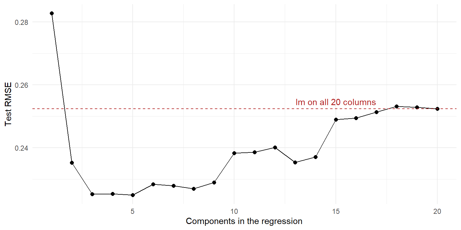
Fit PCR with 1 to 20 components. Score each on test with RMSE. Compare to the 20-column lm.

Code
pcr_rmse <- tibble(M = 1:20) |>
  mutate(rmse = map_dbl(M, \(m) {
    fit <- lm(reformulate(paste0("PC", 1:m), "pps"), data = train_z)
    rmse_vec(test_z$pps, predict(fit, test_z))
  }))

all_rmse <- rmse_vec(test$pps, predict(fit_all, test))

ggplot(pcr_rmse, aes(M, rmse)) +
  geom_line() +
  geom_point(size = 2) +
  geom_hline(yintercept = all_rmse, linetype = "dashed", color = "firebrick") +
  annotate("text", x = 15, y = all_rmse, label = "lm on all 20 columns", vjust = -0.6, color = "firebrick") +
  labs(x = "Components in the regression", y = "Test RMSE") +
  theme_minimal()

  • Test RMSE bottoms out at 3 to 5 components (about 0.225), vs 0.252 for all 20 columns. More than that and it climbs.
  • At \(M = 20\) PCR is the 20-column lm: same columns, rotated.
  • The top few components predict better on new cadets. Same answer as the scree plot, now from prediction.
  • PCA never saw pps. The top components are the biggest patterns in the \(x\)’s. They do not have to be the ones that predict \(y\). Here they are.

Thank You

Thank you for having me in MA376.

Memorial for USMA Class of 2007 classmates: 2LT David R. Lodwick, 2LT Michael R. Girdano, 2LT Andrew N. Caldwell, 2LT Sean P. O'Connor, 1LT Daniel B. Hyde, 1LT Tyler E. Parten, CPT Ian S. Morrison, CPT Sara Knutson Cullen, CPT Jason B. Jones, J Wesley Van Dorn (Honorary Class of '07), MAJ Sean C. Maples, MAJ Eric A. Ewoldsen. And when our work is done, our course on earth is run, may it be said, Well done. Be thou at peace.

Memorial for USMA Class of 2007 classmates: Brandon Stevenson, Ernest Lee, Edward Anderson, Justin Larson. And when our work is done, our course on earth is run, may it be said, Well done. Be thou at peace.