The \(\hat u_j\). Lesson 8’s ridge regression. lmer picks the \(u_j\) that minimize
\[\underbrace{\sum_{i,j} (y_{ij} - \mu - u_j)^2}_{\text{fit the cadets}} \;+\; \underbrace{\lambda \sum_j u_j^2}_{\text{penalty: keep each } u_j \text{ near } 0}\]
- First part: least squares, same as
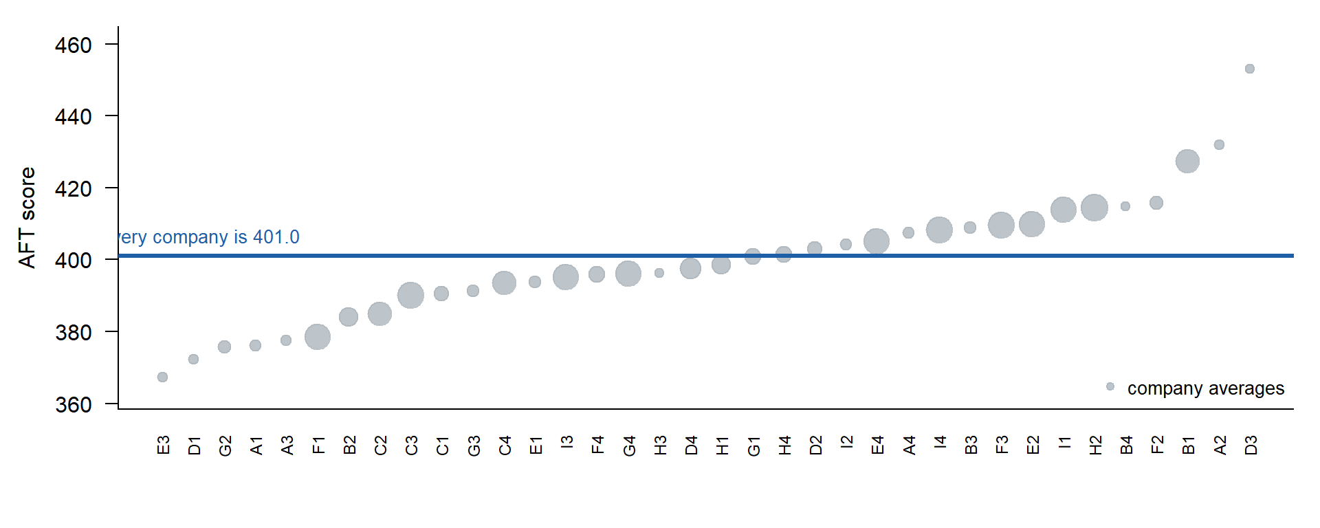
lm. Alone, it gives Model 2: each company its own average.
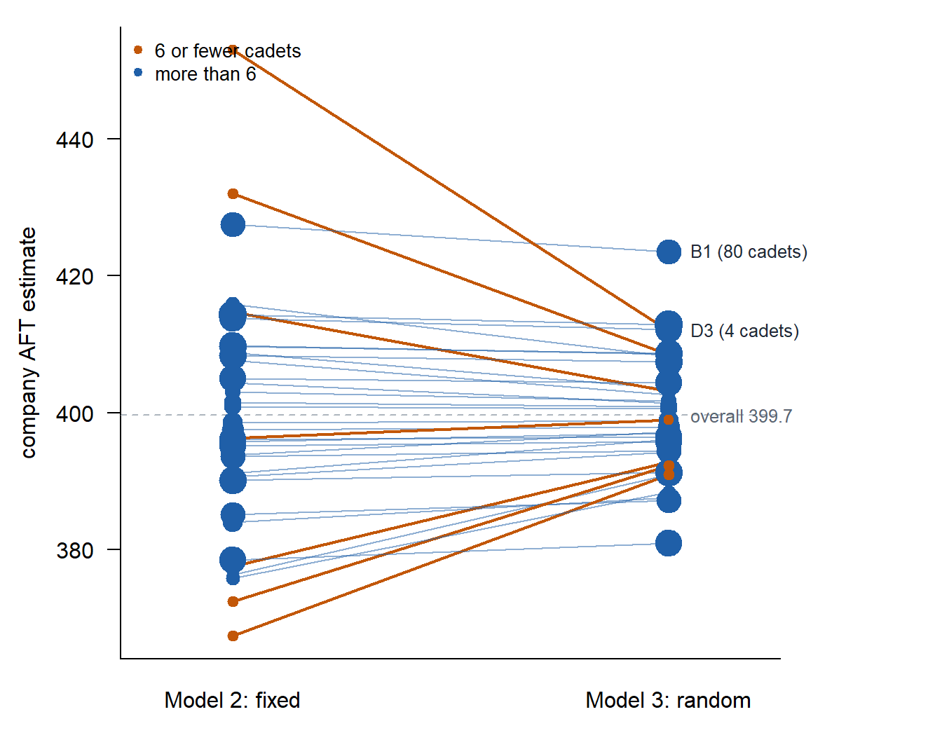
- Second part: a ridge penalty that pulls every \(u_j\) toward 0, the overall average. \(\lambda\) sets how hard.
Solve for one company. Only company \(j\)’s cadets involve \(u_j\):
\[f(u_j) = \sum_{i=1}^{n_j} (y_{ij} - \mu - u_j)^2 + \lambda u_j^2\]
1. Take the derivative.
\[f'(u_j) = -2\sum_{i=1}^{n_j} (y_{ij} - \mu - u_j) + 2\lambda u_j\]
2. Set it to 0. The sum of \(n_j\) cadets’ scores is \(n_j \bar y_j\), so \(\sum_i (y_{ij} - \mu - u_j) = n_j(\bar y_j - \mu - u_j)\):
\[n_j(\bar y_j - \mu - u_j) = \lambda u_j\]
3. Solve for \(u_j\).
\[n_j(\bar y_j - \mu) = (n_j + \lambda)\,u_j \quad\Rightarrow\quad \hat u_j = \frac{n_j}{n_j + \lambda}\,(\bar y_j - \hat\mu)\]
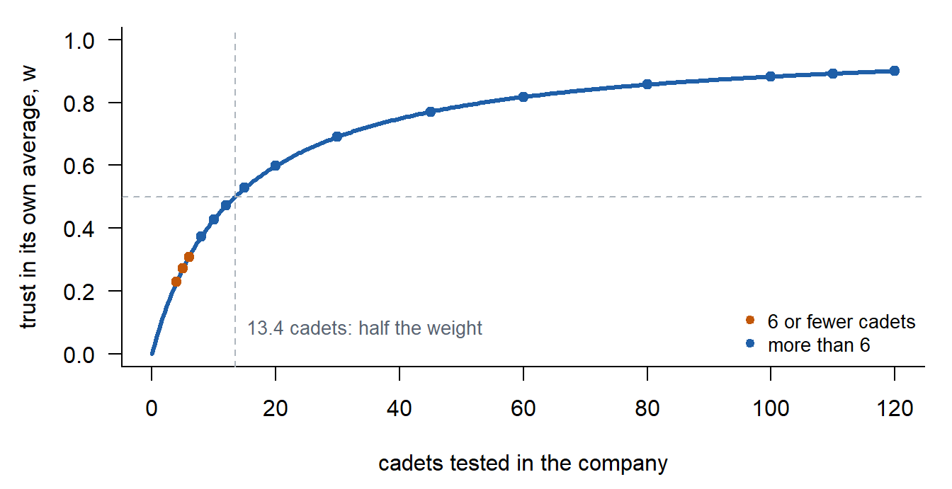
The trust \(w_j\) times the raw gap, as above.
- \(\lambda = 0\), no penalty: \(w_j = 1\), \(\hat u_j\) is the whole raw gap. Model 2.
- \(\lambda\) huge: \(w_j \to 0\), \(\hat u_j \to 0\). Every company is the overall average. Model 1.
- Model 3 sits between, and \(\lambda\) decides where.
Why \(\lambda\) is the variance ratio. Lesson 8 tuned \(\lambda\) by cross-validation. Here the assumption \(u_j \sim N(0, \sigma^2_u)\) sets it. Model 3’s two assumptions, written as \(-2 \log\) density (constants dropped), have two pieces:
\[\underbrace{\frac{1}{\sigma^2}\sum_{i,j}(y_{ij} - \mu - u_j)^2}_{\text{cadets: } \varepsilon \sim N(0, \sigma^2)} + \underbrace{\frac{1}{\sigma^2_u}\sum_j u_j^2}_{\text{companies: } u_j \sim N(0, \sigma^2_u)}\]
Multiply by \(\sigma^2\): the ridge objective with \(\lambda = \sigma^2 / \sigma^2_u\). Ridge had no rule for \(\lambda\). This assumption gives one.
How lmer finds the two variances. By maximum likelihood, with calculus, like Lesson 9’s logistic regression.
1. Write down how likely the data are for any values of the two variances. Company \(j\)’s average has variance \(v_j = \sigma^2_u + \sigma^2 / n_j\): real company spread plus the luck of \(n_j\) cadets. The maximum likelihood (ML) log-likelihood:
\[\ell(\mu, \sigma^2_u, \sigma^2) = -\frac{1}{2}\sum_j \left[ (n_j - 1)\log\sigma^2 + \frac{SS_j}{\sigma^2} + \log v_j + \frac{(\bar y_j - \mu)^2}{v_j} \right] + \text{const}\]
\(SS_j\): the sum of squares of cadets around their own company average.
2. Take the derivative and set it to 0.
\[\frac{\partial \ell}{\partial \sigma^2_u} = -\frac{1}{2}\sum_j \left[ \frac{1}{v_j} - \frac{(\bar y_j - \mu)^2}{v_j^2} \right] = 0\]
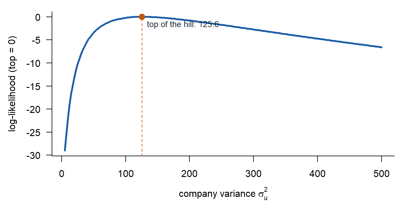
3. No closed-form answer. \(\sigma^2_u\) sits inside every \(v_j\), and each company has its own \(n_j\). You cannot solve it by hand. The computer climbs the hill, as glm did in Lesson 9. lmer uses REML, a version of maximum likelihood with a small correction for estimating \(\mu\): it adds \(-\tfrac{1}{2}\log \sum_j 1/v_j\) to \(\ell\). The hill below is REML.
4. Read off the top. \(\hat\sigma^2_u = 125.6\) and \(\hat\sigma^2 = 1685.3\).