Lesson 26: Model Competition

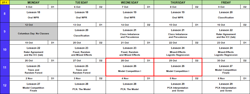
Calendar

Admin

This Lesson

Starter code (the same code as on this page)
Memo 4 data: ma376_leads_m4.csv (12,000 leads, outcomes known) and ma376_leads_score.csv (3,900 incoming, no outcomes)
Leaderboard: https://dustydell.tail280d22.ts.net:8443/ma376 or https://pmid-parent-liquid-nodes.trycloudflare.com/
Your team code: from me, in class

Block 3 Quiz: Lesson 27

In class at Lesson 27: BC2 Fri 30 Oct; A1, BC1 Mon 2 Nov
It covers Lessons 20 to 23. If you can explain these in plain words, you’re ready:
- Why accuracy fools you when the outcome is rare
- What moving the threshold trades, and why 0.5 is a default, not a rule
- Sensitivity, specificity, precision, \(F_1\): what each one counts
- What kappa adds over percent agreement
- The benefit of a random effects model when the groups have small sample sizes

Memo 4

Due Monday 2 November, every section. Hard copy by 1600, in class or at my office, TH239B.
Tasking, data description
Memo 4 is individual. Use your team’s model if you like; the argument is yours.

Coming Up

Capstone Milestone 2: methodology and preliminary results. Due 2359 Friday 13 November, 60 points.
Capstone final presentation. Lessons 37 and 38, 3 to 8 December, 100 points.
I’m here through Lesson 29, 6 November.

TEE Slots

All TEE periods run 0730 to 1100. Find your name under your section.

MA376 A1 14 (15 cadets)

P1: Tue 15 Dec (8)	P4: Wed 16 Dec (7)
Anteen	Baron
Carroll	Fountain
Cole	Hardwick
Fonte	Rebolledo
Konopka	Shioutakon
Ploetz	Smith
Sun	Youmans
Toth

MA376 BC1 15 (14 cadets)

P1: Tue 15 Dec (5)	P4: Wed 16 Dec (9)
Bode	Best
Lee	De La Torre
Ndiaye	Laub
O’Keefe	Loughman
Russell	Miranda
	Nguyen
	Plummer
	Ward
	Weisenborn

MA376 BC2 16 (15 cadets)

P1: Tue 15 Dec (4)	P4: Wed 16 Dec (11)
Gray	Applegate
Harris	Cannon
Van Kley	Ivey
Zhai	Johnson
	Kendig
	Marino
	Myers
	Silverman
	Song
	Tullier
	Wittrock

Break!

Ten softball players lined up arm in arm on a lit field at night, each in a different colored shirt with a white letter m, like a bag of M&Ms.

What We Did: Lessons 20 to 25

Review: Judging a Classifier (Lesson 20)

	Truth positive	Truth negative
Predicted positive	TP	FP, a false alarm
Predicted negative	FN, a miss	TN

Accuracy \(= \dfrac{TP + TN}{n}\)
Sensitivity (recall) \(= \dfrac{TP}{TP + FN}\), specificity \(= \dfrac{TN}{TN + FP}\)
Precision \(= \dfrac{TP}{TP + FP}\)
\(F_1 = \dfrac{2\,TP}{2\,TP + FP + FN}\)
Cut probabilities into labels at a threshold. \(0.5\) is a default, not a rule.

Review: Class Imbalance and Prevalence (Lesson 21)

Rare outcome: the null classifier scores \(1 - \text{prevalence}\), and a \(0.5\) threshold flags almost nothing.
Three fixes: move the threshold, class weights (glm(..., weights = w)), undersample. Each one moves the cutoff. None improves the model.
Sensitivity and specificity do not move with prevalence. Precision does.
Report performance with the prevalence it was measured at.

Review: Rater Agreement and the ICC (Lesson 22)

Percent agreement \(p_o\). Chance agreement \(p_e = P(A)P(B) + P(A^c)P(B^c)\)
Cohen’s kappa \(\kappa = \dfrac{p_o - p_e}{1 - p_e}\): agreement once you remove chance. Falls as prevalence moves to an extreme.
\(\text{PABAK} = 2p_o - 1\): kappa with the prevalence set at half
ICC \(= \dfrac{\hat\sigma^2_{\text{subject}}}{\hat\sigma^2_{\text{subject}} + \hat\sigma^2_{\text{rater}} + \hat\sigma^2_{\text{error}}}\), from a two-way ANOVA with raters as blocks
Reliability is not validity: raters can agree and all be wrong.

Review: Fixed, Random and Mixed Effects (Lesson 23)

\(y_{ij} = \mu + u_j + \varepsilon_{ij}\), \(u_j \sim N(0, \sigma^2_u)\), \(\varepsilon_{ij} \sim N(0, \sigma^2)\)
lmer(y ~ 1 + (1 | group), data = d), then fixef(), ranef(), coef()
\(\hat y_{ij} = \hat\mu + w_j(\bar y_j - \hat\mu)\), \(w_j = \dfrac{n_j}{n_j + \lambda}\), \(\lambda = \dfrac{\hat\sigma^2}{\hat\sigma^2_u}\): small groups shrink toward the average
\(\text{ICC} = \dfrac{\hat\sigma^2_u}{\hat\sigma^2_u + \hat\sigma^2}\)
Fixed: these levels are all you care about. Random: the levels are a sample of many.

Review: Mixed-Effects Logistic Regression (Lesson 24)

\(\log\dfrac{p_{ij}}{1 - p_{ij}} = \mu + u_j\), \(u_j \sim N(0, \sigma^2_u)\). No \(\varepsilon\): pass or fail is the noise.
glmer(y ~ x + (1 | group), family = binomial, data = d)
predict(fit, newdata, type = "response", allow.new.levels = TRUE)
glm with a dummy per group: a group at 100% gets \(\hat\beta \to \infty\). glmer shrinks it.
\(\text{ICC} = \dfrac{\hat\sigma^2_u}{\hat\sigma^2_u + \pi^2/3}\)

Review: Trees and Random Forest (Lesson 25)

A tree splits the data into boxes. Each split picks the predictor and cut that lowers Gini impurity the most.
Gini for a box: \(G = 2p(1 - p)\). After a split, average the two boxes, weighted by size.
A tree grown all the way memorizes the training data and does worse on new data. Limit it.
Random forest: many trees, each on a bootstrap sample, each split choosing from mtry random predictors. The forest votes.
randomForest(y ~ ., data = train, ntree = , mtry = , nodesize = ); tune on out-of-bag \(F_1\).
predict(fit, newdata, type = "prob") gives the share of trees that vote yes.
Variable importance says which predictors the forest leans on, not how.

What We’re Doing: Lesson 26

Today we build the models behind Memo 4 to Mr. Lemmes. Your memo needs a rule that scores every incoming lead. Your team builds and tests that rule today; the leaderboard tells you how well it ranks.

The Tasking

Mr. Lemmes, Memo 4:

The battalion now takes in 3,900 leads a week.
205 recruiters can each open about 6 new leads a week: \(205 \times 6 = 1{,}230\) calls.
The other 2,670 leads never get a call.
“Build a rule that scores an incoming lead, and tell me where to draw the line.”

	Today, with your team	Memo 4, on your own
The question	Which model and cut score best?	Where do we draw the line?
The answer	A model and its probabilities	A recommendation to Mr. Lemmes
Judged by	The leaderboard (not graded)	The memo rubric (graded)

The Data

Install anything you don’t have, then load it.

pkgs <- c("tidyverse", "yardstick", "lme4", "randomForest", "ggrepel")
install.packages(setdiff(pkgs, rownames(installed.packages())))

library(tidyverse)
library(yardstick)
library(lme4)
library(randomForest)
library(ggrepel)

Both Memo 4 files from Canvas go in the same folder as your script. In RStudio: Session > Set Working Directory > To Source File Location.

leads    <- read_csv("ma376_leads_m4.csv", show_col_types = FALSE) |>
  mutate(across(where(is.character), factor), enlisted = factor(enlisted))
incoming <- read_csv("ma376_leads_score.csv", show_col_types = FALSE) |>
  mutate(across(where(is.character), factor))

head(leads) |> print(width = Inf)

# A tibble: 6 × 9
  station market_type propensity lead_source  education      age distance_miles social_media enlisted
  <fct>   <fct>            <dbl> <fct>        <fct>        <dbl>          <dbl> <fct>        <fct>   
1 Marion  Frontier           107 online ad    HS grad         19             11 Yes          0       
2 Ashford Urban               85 online ad    HS grad         19             14 No           0       
3 Alton   Rural              117 school event HS grad         20             14 Yes          0       
4 Jasper  Urban               89 walk-in      HS grad         21             50 Yes          0       
5 Lamont  Rural              111 referral     Some college    19             19 No           0       
6 Redmond Suburban           106 online ad    HS senior       19             27 Yes          0

leads |> count(enlisted) |> mutate(share = n / sum(n))

# A tibble: 2 × 3
  enlisted     n  share
  <fct>    <int>  <dbl>
1 0        11684 0.974 
2 1          316 0.0263

Worked leads: 12,000, outcome known. 2.6% enlisted.
Incoming: 3,900, no enlisted column. You predict those.
lead_id ties your prediction to a lead. Never drop it or sort it away.

Exploratory Data Analysis

Every plot: the share of leads that enlisted. Dashed line: the overall 2.6%. Bars: 95% intervals.

Code

leads |>
  group_by(lead_source) |>
  summarise(n = n(), rate = mean(enlisted == "1")) |>
  mutate(se = sqrt(rate * (1 - rate) / n), lead_source = fct_reorder(lead_source, rate)) |>
  ggplot(aes(x = rate, y = lead_source)) +
  geom_vline(xintercept = base, linetype = "dashed", color = gold, linewidth = 0.9) +
  geom_errorbarh(aes(xmin = rate - 1.96 * se, xmax = rate + 1.96 * se), height = 0.2, color = navy) +
  geom_point(size = 4, color = navy) +
  geom_text(aes(label = paste0(scales::percent(rate, 0.1), "  (", scales::comma(n), " leads)")),
            vjust = -1.2, size = 4) +
  scale_x_continuous(labels = scales::percent) +
  labs(title = "Referrals enlist almost twice as often as online ads", x = "Enlisted", y = NULL)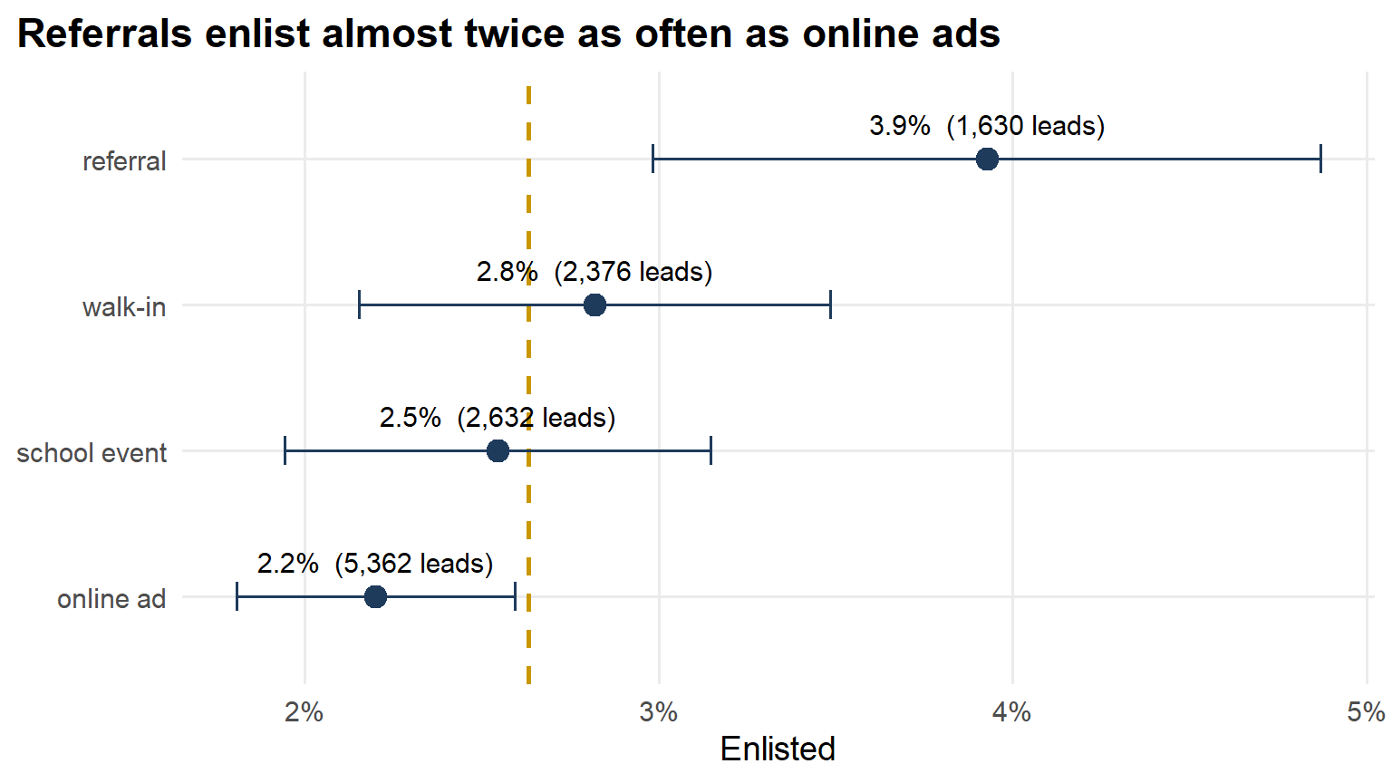

Code

leads |>
  group_by(education) |>
  summarise(n = n(), rate = mean(enlisted == "1")) |>
  mutate(se = sqrt(rate * (1 - rate) / n), education = fct_reorder(education, rate)) |>
  ggplot(aes(x = rate, y = education)) +
  geom_vline(xintercept = base, linetype = "dashed", color = gold, linewidth = 0.9) +
  geom_errorbarh(aes(xmin = rate - 1.96 * se, xmax = rate + 1.96 * se), height = 0.2, color = navy) +
  geom_point(size = 4, color = navy) +
  geom_text(aes(label = paste0(scales::percent(rate, 0.1), "  (", scales::comma(n), " leads)")),
            vjust = -1.2, size = 4) +
  scale_x_continuous(labels = scales::percent) +
  labs(title = "High school seniors enlist most", x = "Enlisted", y = NULL)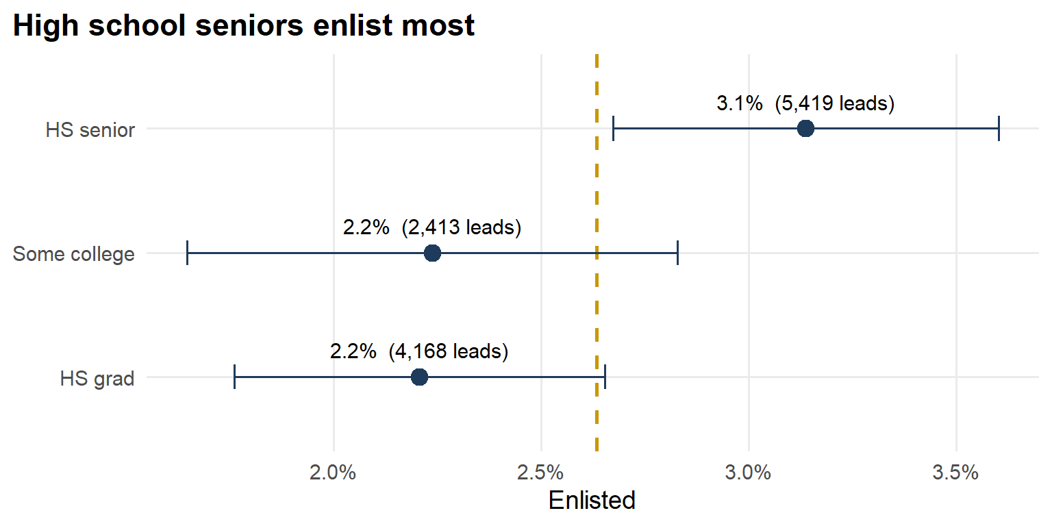

Code

leads |>
  group_by(lead_source, education) |>
  summarise(n = n(), rate = mean(enlisted == "1"), .groups = "drop") |>
  ggplot(aes(x = education, y = fct_reorder(lead_source, rate), fill = rate)) +
  geom_tile(color = "white", linewidth = 1.5) +
  geom_text(aes(label = paste0(scales::percent(rate, 0.1), "\n", n, " leads"),
                color = rate > 0.04), size = 4, show.legend = FALSE) +
  scale_fill_gradient(low = "#eef2f7", high = navy, labels = scales::percent) +
  scale_color_manual(values = c("black", "white")) +
  labs(title = "The best cell: a referral who is still in high school",
       x = NULL, y = NULL, fill = "Enlisted") +
  theme(panel.grid = element_blank(), legend.key.width = unit(2, "cm"))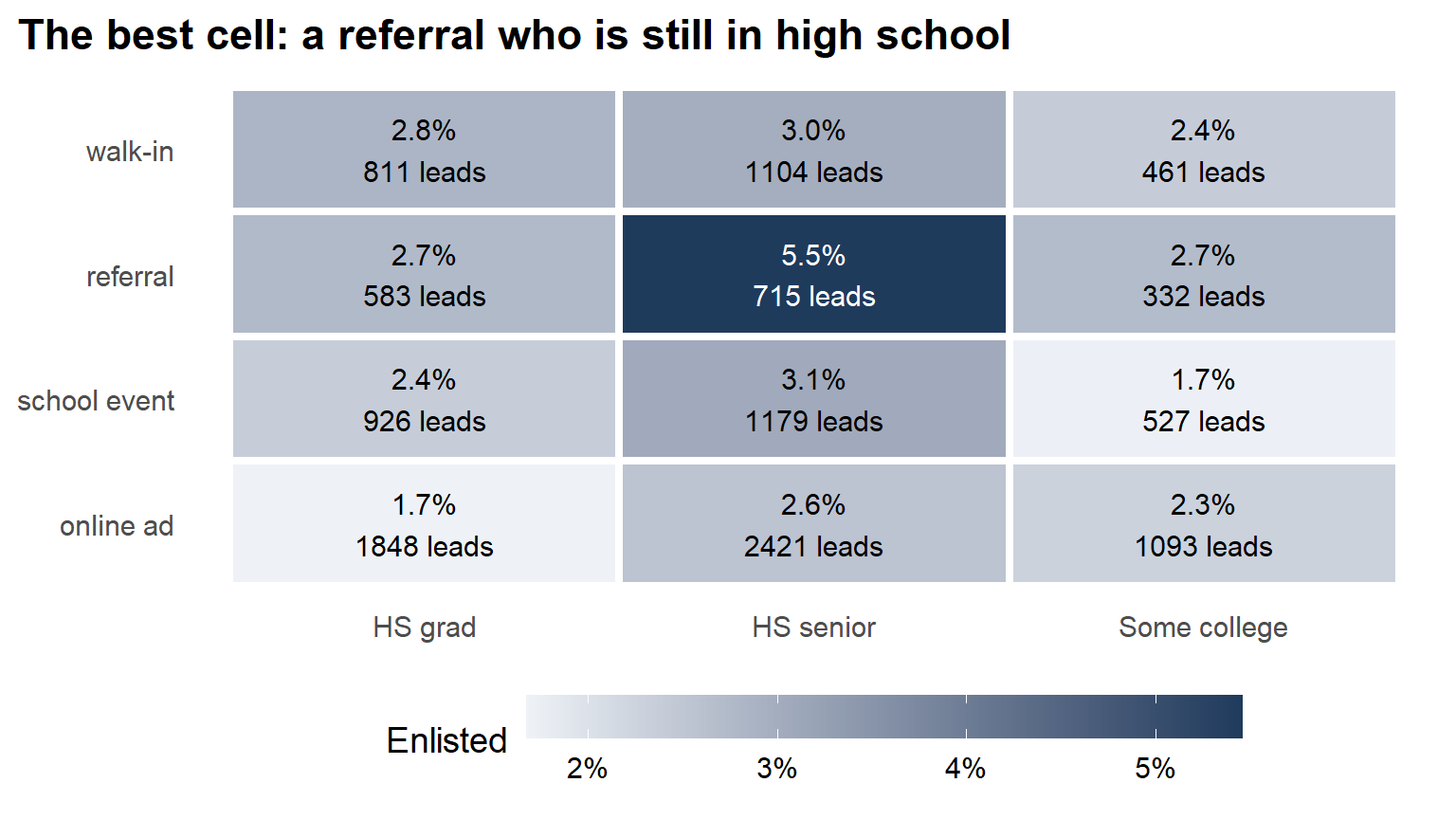

Code

leads |>
  group_by(age) |>
  summarise(n = n(), rate = mean(enlisted == "1")) |>
  mutate(se = sqrt(rate * (1 - rate) / n)) |>
  ggplot(aes(x = age, y = rate)) +
  overall +
  geom_errorbar(aes(ymin = pmax(rate - 1.96 * se, 0), ymax = rate + 1.96 * se), width = 0.2, color = navy) +
  geom_point(aes(size = n), color = navy) +
  scale_y_continuous(labels = scales::percent) +
  scale_x_continuous(breaks = 17:24) +
  scale_size_area(max_size = 8, labels = scales::comma) +
  labs(title = "Age: no clear pattern. Watch the small groups at the end",
       x = "Age", y = "Enlisted", size = "Leads")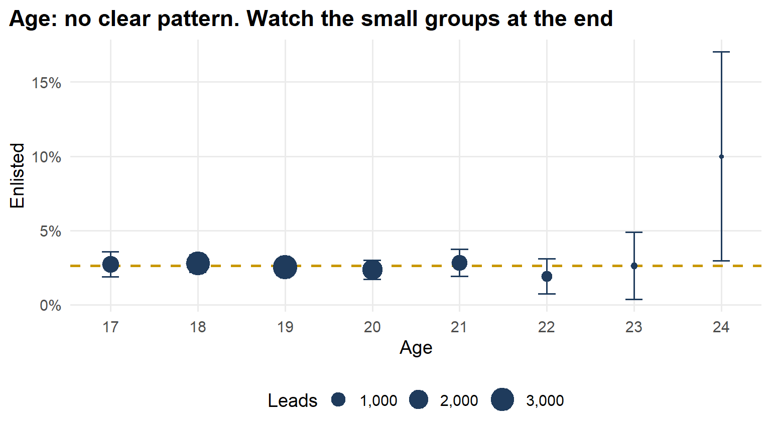

Code

leads |>
  group_by(station, market_type, propensity) |>
  summarise(n = n(), rate = mean(enlisted == "1"), .groups = "drop") |>
  ggplot(aes(x = propensity, y = rate)) +
  overall +
  geom_smooth(method = "lm", se = FALSE, color = "gray40", linewidth = 0.8) +
  geom_point(aes(size = n, color = market_type), alpha = 0.8) +
  scale_y_continuous(labels = scales::percent) +
  scale_color_manual(values = c(Frontier = gold, Rural = "#6b8e23", Suburban = "#7a9cc6", Urban = navy)) +
  scale_size_area(max_size = 6, guide = "none") +
  labs(title = "Propensity belongs to the station: one dot per station",
       x = "Home-market propensity", y = "Enlisted", color = NULL)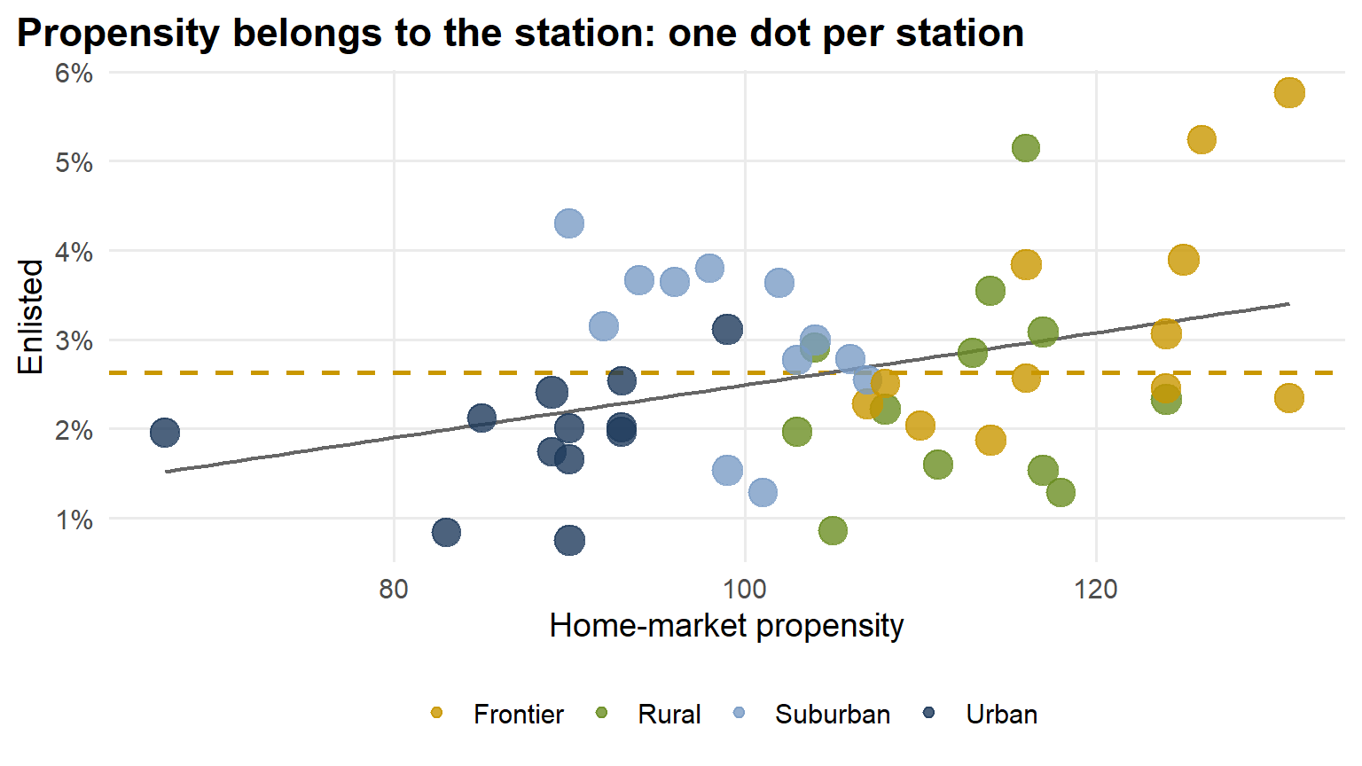

Code

stations <- leads |>
  group_by(station) |>
  summarise(n = n(), rate = mean(enlisted == "1"))

funnel <- tibble(n = seq(min(stations$n) - 20, max(stations$n) + 20)) |>
  mutate(lo = base - 1.96 * sqrt(base * (1 - base) / n), hi = base + 1.96 * sqrt(base * (1 - base) / n))

ggplot() +
  geom_ribbon(data = funnel, aes(x = n, ymin = pmax(lo, 0), ymax = hi), fill = navy, alpha = 0.12) +
  geom_hline(yintercept = base, linetype = "dashed", color = gold, linewidth = 0.9) +
  geom_point(data = stations, aes(x = n, y = rate), color = navy, size = 3) +
  ggrepel::geom_text_repel(data = stations |> filter(rate == max(rate) | rate == min(rate)),
                           aes(x = n, y = rate, label = station), size = 4) +
  scale_y_continuous(labels = scales::percent) +
  labs(title = paste(n_station, "stations. Shaded: where luck alone puts a station"),
       x = "Leads at the station", y = "Enlisted")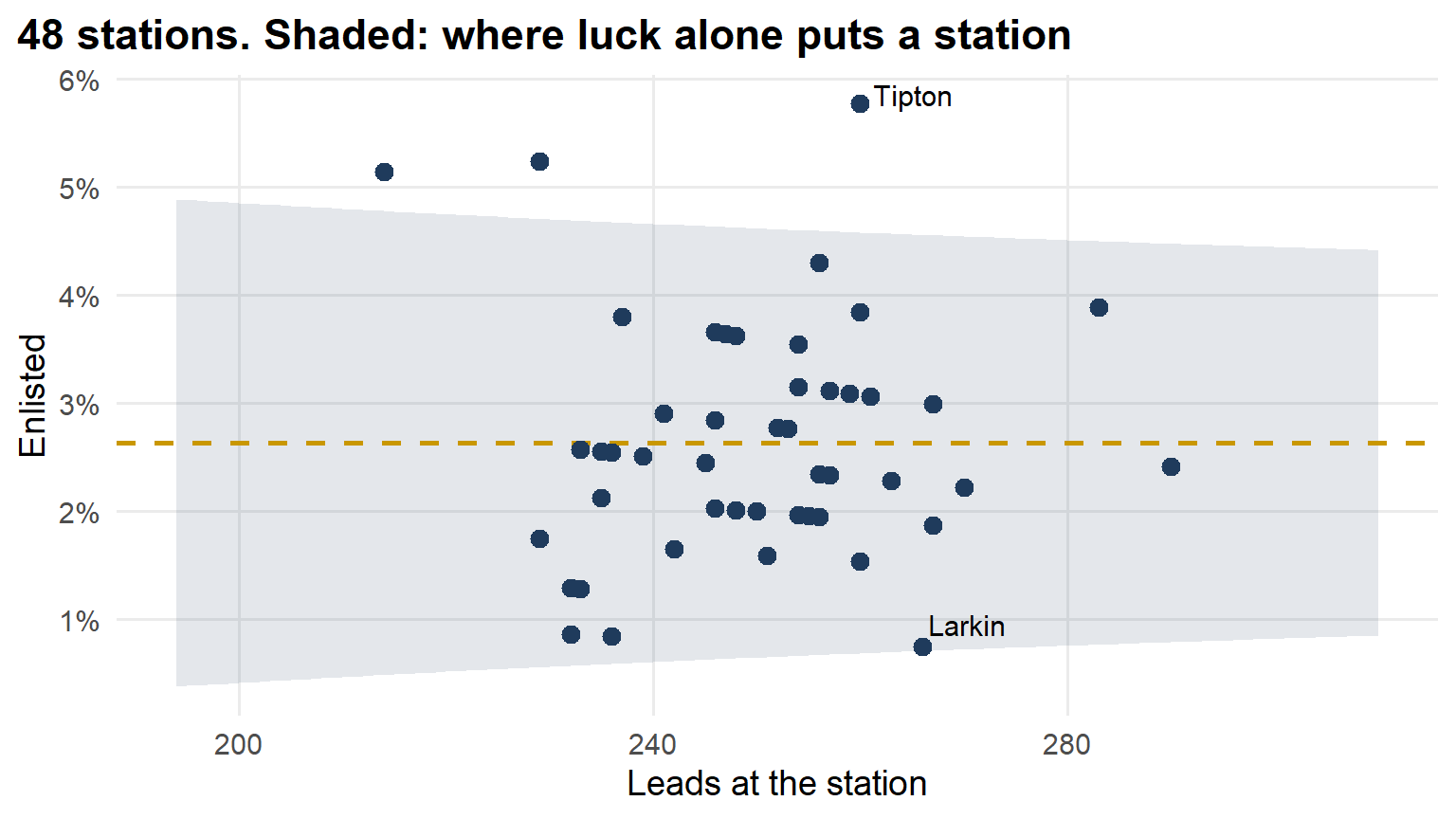

Code

bind_rows(
  leads |> mutate(group = cut(distance_miles, c(0, 10, 20, 30, 40, 50, 60), labels = c("0-10", "11-20", "21-30", "31-40", "41-50", "51-60")),
                  panel = "Miles from the station"),
  leads |> mutate(group = factor(social_media), panel = "On social media")
) |>
  group_by(panel, group) |>
  summarise(n = n(), rate = mean(enlisted == "1"), .groups = "drop") |>
  mutate(se = sqrt(rate * (1 - rate) / n)) |>
  ggplot(aes(x = group, y = rate)) +
  overall +
  geom_errorbar(aes(ymin = rate - 1.96 * se, ymax = rate + 1.96 * se), width = 0.2, color = navy) +
  geom_point(size = 3.5, color = navy) +
  facet_wrap(~ panel, scales = "free_x") +
  scale_y_continuous(labels = scales::percent) +
  labs(title = "Two predictors that may do nothing", x = NULL, y = "Enlisted")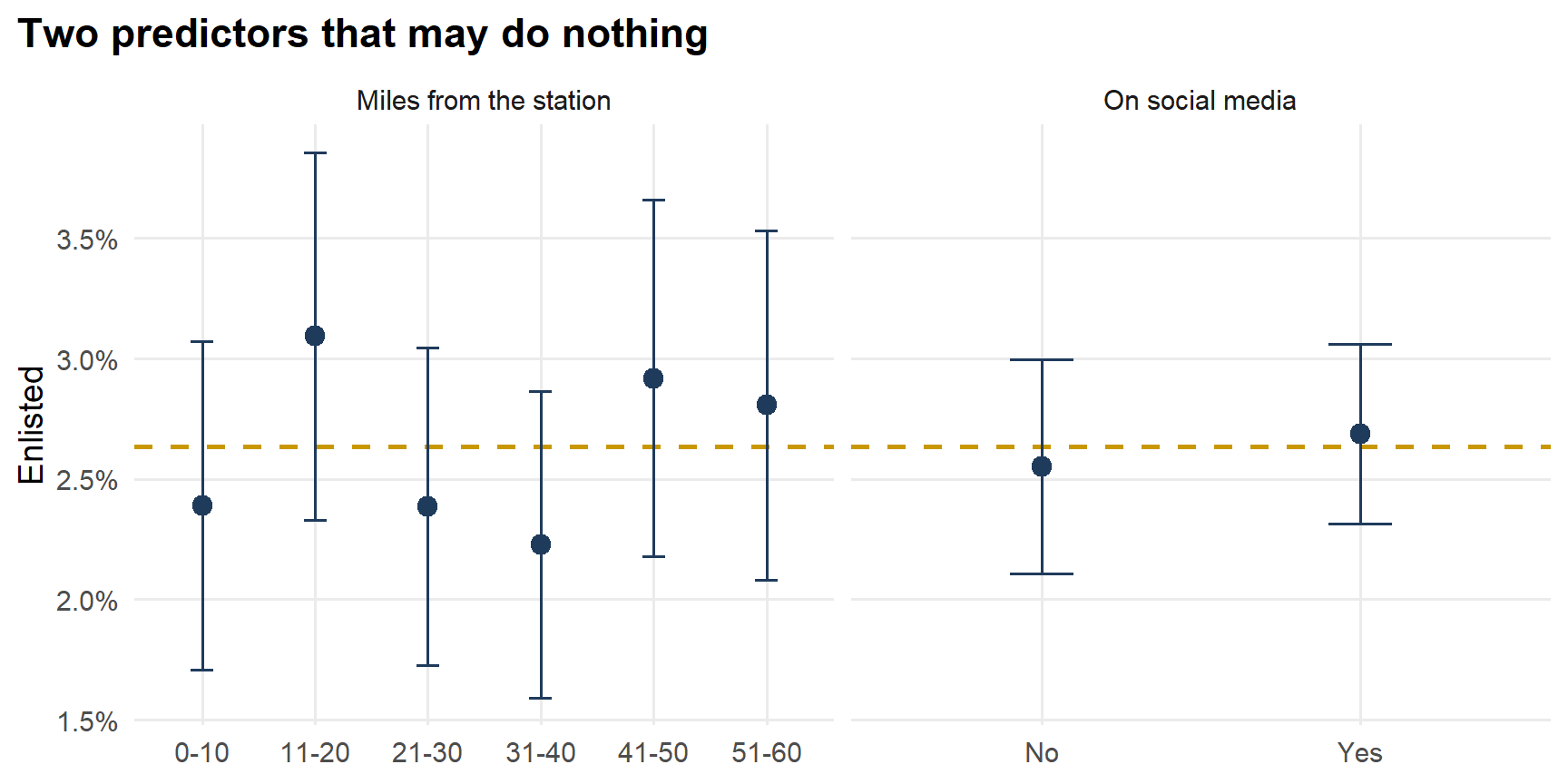

The Competition

Six model types. Your team can upload one of each. Use your best model for Memo 4.

	Model type	From	Your cut
1	Logistic regression	Lessons 9, 20	0.5
2	Logistic, your cut (Fix 1)	Lesson 21	Yours
3	Logistic, class weights (Fix 2)	Lesson 21	Yours
4	Logistic, undersampled (Fix 3)	Lesson 21	Yours
5	Mixed-effects logistic	Lesson 24	Yours
6	Random forest	Lesson 25	Yours

In your teams. One team code per team.
Upload: a CSV with three columns: lead_id, probability, and call (1 = a recruiter calls this lead, 0 = not). Exactly 3,900 rows, each lead once. Pick the model type when you upload at the leaderboard.
Score: \(F_1\) on your call column. Highest \(F_1\) wins each model type.
The board shows every team’s latest upload of every type. Filter by model type. Sort by any column: \(F_1\), accuracy, sensitivity, specificity, precision, calls, enlistees caught.
Live board: scores a hidden 30% of the incoming leads. Final board: scores the other 70%, revealed at Lesson 27.
Five uploads per model type per day.
Ties: the earlier upload wins.
Data: Memo 4 files only. No outside data. Talk methods with other teams; don’t share code.
The board closes Thursday 29 October at 2359, every section.
Not graded. Bragging rights.

How You’re Scored

Your call column against what happened:

	Enlisted	Did not enlist
Called	TP, caught	FP, a call that went nowhere
Not called	FN, left unworked	TN

\(F_1 = \dfrac{2\,TP}{2\,TP + FP + FN}\): the score.
Accuracy is on the board too. Sort by it and look at what lands on top.
Calls \(= TP + FP\). The recruiters can make 1,230. The board shows yours.
Enlistees caught \(= TP\).

Starter Code: Model Type 1

Logistic regression, cut at 0.5. This is the baseline. Beat it.

1. Split the Worked Leads

The board only scores incoming leads, and you get five uploads a day. Check your models here first.

set.seed(376)
leads <- leads |> mutate(set = if_else(runif(n()) < 0.7, "train", "test"))
train <- leads |> filter(set == "train") |> select(-set)
test  <- leads |> filter(set == "test")  |> select(-set)

2. Fit It

station is left out: 48 towns would be 47 dummies. Lesson 24 has a better idea.

fit_logit <- glm(enlisted ~ market_type + propensity + lead_source + education + age +
                   distance_miles + social_media,
                 family = binomial, data = train)
summary(fit_logit)


Call:
glm(formula = enlisted ~ market_type + propensity + lead_source + 
    education + age + distance_miles + social_media, family = binomial, 
    data = train)

Coefficients:
                         Estimate Std. Error z value Pr(>|z|)    
(Intercept)             -5.693738   1.474972  -3.860 0.000113 ***
market_typeRural        -0.249938   0.200062  -1.249 0.211554    
market_typeSuburban      0.170078   0.265042   0.642 0.521067    
market_typeUrban        -0.087425   0.357716  -0.244 0.806922    
propensity               0.009914   0.009747   1.017 0.309111    
lead_sourcereferral      0.586756   0.189268   3.100 0.001934 ** 
lead_sourceschool event  0.241696   0.177601   1.361 0.173548    
lead_sourcewalk-in       0.347640   0.176793   1.966 0.049257 *  
educationHS senior       0.430638   0.153911   2.798 0.005142 ** 
educationSome college    0.117872   0.200103   0.589 0.555823    
age                      0.028375   0.044970   0.631 0.528064    
distance_miles           0.002397   0.003898   0.615 0.538654    
social_mediaYes          0.104913   0.136557   0.768 0.442326    
---
Signif. codes:  0 '***' 0.001 '**' 0.01 '*' 0.05 '.' 0.1 ' ' 1

(Dispersion parameter for binomial family taken to be 1)

    Null deviance: 2149.8  on 8372  degrees of freedom
Residual deviance: 2121.9  on 8360  degrees of freedom
AIC: 2147.9

Number of Fisher Scoring iterations: 6

3. Predict, and Cut at 0.5

results_logit <- test |>
  mutate(prob = predict(fit_logit, test, type = "response"),
         call = factor(if_else(prob > 0.5, 1, 0), levels = c(0, 1)))

4. Score It Like the Board

conf_mat(results_logit, truth = enlisted, estimate = call)

          Truth
Prediction    0    1
         0 3547   80
         1    0    0

lead_metrics <- metric_set(f_meas, accuracy, sensitivity, specificity, precision)

results_logit |>
  lead_metrics(truth = enlisted, estimate = call, event_level = "second")

# A tibble: 5 × 3
  .metric     .estimator .estimate
  <chr>       <chr>          <dbl>
1 f_meas      binary        NA    
2 accuracy    binary         0.978
3 sensitivity binary         0    
4 specificity binary         1    
5 precision   binary        NA

\(F_1\) is NA: no calls, so precision is \(0/0\). The board scores it 0.
97% accurate, and not one enlistee caught.

5. Refit on All 12,000 and Write the Upload

fit_final <- glm(enlisted ~ market_type + propensity + lead_source + education + age +
                   distance_miles + social_media,
                 family = binomial, data = leads)

upload <- incoming |>
  mutate(probability = predict(fit_final, incoming, type = "response"),
         call = if_else(probability > 0.5, 1, 0)) |>
  select(lead_id, probability, call)

head(upload)

# A tibble: 6 × 3
  lead_id probability  call
    <dbl>       <dbl> <dbl>
1       1      0.0245     0
2       2      0.0272     0
3       3      0.0237     0
4       4      0.0246     0
5       5      0.0126     0
6       6      0.0171     0

nrow(upload)

[1] 3900

write_csv(upload, "team_XX_type1.csv")

Put your team code in place of XX. Upload it as model type 1. That’s your team on the board.

Your Turn: Model Types 2 to 6

Each type runs start to finish, the same five steps as type 1: fit on train, predict test, score it, refit on all 12,000, predict the incoming leads and write the upload. Fill in the blanks, run it, upload it, then make it better.

Type 2: Logistic, Your Cut (Fix 1)

Pick your predictors. Tune the cut on \(F_1\) by five-fold cross-validation on train, as in Lesson 21. Never tune on test.

cuts <- seq(0.01, 0.10, by = 0.005)                  # the cuts to try
set.seed(11)
fold <- sample(rep(1:5, length.out = nrow(train)))   # each training lead gets a fold
p_cv <- numeric(nrow(train))
for (k in 1:5) {
  f <- glm(enlisted ~ ___,
           family = binomial, data = train[fold != k, ])                  # fit on four folds
  p_cv[fold == k] <- predict(f, train[fold == k, ], type = "response")    # predict the fifth
}

f1 <- sapply(cuts, function(t) {
  call <- p_cv > t
  2 * sum(call & train$enlisted == "1") / (sum(call) + sum(train$enlisted == "1"))
})
best_cut <- cuts[which.max(f1)]
best_cut

fit_cut <- glm(enlisted ~ ___,
               family = binomial, data = train)

results_cut <- test |>
  mutate(prob = predict(fit_cut, test, type = "response"),
         call = factor(if_else(prob > best_cut, 1, 0), levels = c(0, 1)))

results_cut |> conf_mat(truth = enlisted, estimate = call)
results_cut |> lead_metrics(truth = enlisted, estimate = call, event_level = "second")

fit_cut_final <- glm(enlisted ~ ___,
                     family = binomial, data = leads)

upload <- incoming |>
  mutate(probability = predict(fit_cut_final, incoming, type = "response"),
         call = if_else(probability > best_cut, 1, 0)) |>
  select(lead_id, probability, call)

sum(upload$call)
write_csv(upload, "team_XX_type2.csv")

The cut is a choice. Best \(F_1\) is one reason. 1,230 calls is another.

Type 3: Logistic, Class Weights (Fix 2)

Each training enlistee counts as \(n_0 / n_1\) leads, as in Lesson 21. Cut at 0.5.

w <- ifelse(train$enlisted == "1", sum(train$enlisted == "0") / sum(train$enlisted == "1"), 1)
fit_weighted <- glm(enlisted ~ ___,
                    family = binomial, data = train, weights = w)
# R warns about "non-integer #successes" because the weights aren't whole numbers. We mean it.

results_weighted <- test |>
  mutate(prob = predict(fit_weighted, test, type = "response"),
         call = factor(if_else(prob > 0.5, 1, 0), levels = c(0, 1)))

results_weighted |> conf_mat(truth = enlisted, estimate = call)
results_weighted |> lead_metrics(truth = enlisted, estimate = call, event_level = "second")

w_all <- ifelse(leads$enlisted == "1", sum(leads$enlisted == "0") / sum(leads$enlisted == "1"), 1)
fit_weighted_final <- glm(enlisted ~ ___,
                          family = binomial, data = leads, weights = w_all)

upload <- incoming |>
  mutate(probability = predict(fit_weighted_final, incoming, type = "response"),
         call = if_else(probability > 0.5, 1, 0)) |>
  select(lead_id, probability, call)

sum(upload$call)
write_csv(upload, "team_XX_type3.csv")

How many does it call at 0.5? Compare to 1,230.

Type 4: Logistic, Undersampled (Fix 3)

In train, keep every enlistee and the same number of leads that didn’t enlist, drawn at random, as in Lesson 21. Cut at 0.5.

set.seed(376)
keep <- c(which(train$enlisted == "1"), sample(which(train$enlisted == "0"), sum(train$enlisted == "1")))
fit_under <- glm(enlisted ~ ___,
                 family = binomial, data = train[keep, ])

results_under <- test |>
  mutate(prob = predict(fit_under, test, type = "response"),
         call = factor(if_else(prob > 0.5, 1, 0), levels = c(0, 1)))

results_under |> conf_mat(truth = enlisted, estimate = call)
results_under |> lead_metrics(truth = enlisted, estimate = call, event_level = "second")

set.seed(376)
keep_all <- c(which(leads$enlisted == "1"), sample(which(leads$enlisted == "0"), sum(leads$enlisted == "1")))
fit_under_final <- glm(enlisted ~ ___,
                       family = binomial, data = leads[keep_all, ])

upload <- incoming |>
  mutate(probability = predict(fit_under_final, incoming, type = "response"),
         call = if_else(probability > 0.5, 1, 0)) |>
  select(lead_id, probability, call)

sum(upload$call)
write_csv(upload, "team_XX_type4.csv")

Type 5: Mixed-Effects Logistic (Lesson 24)

Your predictors plus a random intercept for each station, fit with glmer as in Lesson 24. A 0.5 cut calls nobody again, so use type 2’s cut.

fit_glmer <- glmer(enlisted ~ ___ + (1 | station),
                   family = binomial, data = train)
summary(fit_glmer)

results_glmer <- test |>
  mutate(prob = predict(fit_glmer, test, type = "response", allow.new.levels = TRUE),
         call = factor(if_else(prob > best_cut, 1, 0), levels = c(0, 1)))

results_glmer |> conf_mat(truth = enlisted, estimate = call)
results_glmer |> lead_metrics(truth = enlisted, estimate = call, event_level = "second")

fit_glmer_final <- glmer(enlisted ~ ___ + (1 | station),
                         family = binomial, data = leads)

upload <- incoming |>
  mutate(probability = predict(fit_glmer_final, incoming, type = "response", allow.new.levels = TRUE),
         call = if_else(probability > best_cut, 1, 0)) |>
  select(lead_id, probability, call)

sum(upload$call)
write_csv(upload, "team_XX_type5.csv")

Look at the station variance. What is it telling you?
Its own cut: run type 2’s loop with this glmer in place of glm. Five glmer fits take a minute or two.
If glmer warns about converging or rescaling, that’s the size of propensity and distance_miles. Try scale().
allow.new.levels = TRUE: a station with no worked leads gets the average station.

Type 6: Random Forest (Lesson 25)

Fit the forest as in Lesson 25. A majority vote calls nobody here, so cut the share of trees that vote “enlisted.” Tune the cut on the out-of-bag votes, never on test.

set.seed(376)
fit_rf <- randomForest(enlisted ~ ___,
                       data = train,
                       ntree = ___,       # how many trees
                       mtry = ___,        # predictors each split may look at
                       nodesize = ___)    # smallest box a tree can make
fit_rf

p_oob <- fit_rf$votes[, "1"]   # each training lead, voted on only by trees that never saw it

f1_rf <- sapply(cuts, function(t) {
  call <- p_oob > t
  2 * sum(call & train$enlisted == "1") / (sum(call) + sum(train$enlisted == "1"))
})
best_rf <- cuts[which.max(f1_rf)]
best_rf

results_rf <- test |>
  mutate(prob = predict(fit_rf, test, type = "prob")[, "1"],
         call = factor(if_else(prob > best_rf, 1, 0), levels = c(0, 1)))

results_rf |> conf_mat(truth = enlisted, estimate = call)
results_rf |> lead_metrics(truth = enlisted, estimate = call, event_level = "second")

set.seed(376)
fit_rf_final <- randomForest(enlisted ~ ___,
                             data = leads, ntree = ___, mtry = ___, nodesize = ___)

upload <- incoming |>
  mutate(probability = predict(fit_rf_final, incoming, type = "prob")[, "1"],
         call = if_else(probability > best_rf, 1, 0)) |>
  select(lead_id, probability, call)

sum(upload$call)
write_csv(upload, "team_XX_type6.csv")

Tune ntree, mtry, nodesize with Lesson 25’s grid. Check the winner on test before you upload: with this few enlistees, the best OOB score can be luck.

From the Board to the Memo

The board answers one question: which model and cut score best? Memo 4 asks the rest. Your memo should answer:

How many future Soldiers are below your line each week?
What would it take to reach them?
Is 6 new leads per recruiter the right capacity? What happens to your answer at 5, or 8?
Your model trained on leads from before the surge. Should Mr. Lemmes trust it on the leads after?

Before Lesson 27

The board closes Thursday 29 October at 2359.
Block 3 quiz, in class at Lesson 27 (BC2 Fri 30 Oct; A1, BC1 Mon 2 Nov). Lessons 20 to 23; the list is in the Admin above.
Lesson 27: the final board, and what the winners did.
Memo 4 due Monday 2 November, hard copy by 1600.